Quantum Regression and Time Series
This page shows complete regression runs with HQNR and QSVR, and time-series
forecasting with QuantumTimeSeriesRegressor.
Data
from eigenkit.datasets import load_dataset
from sklearn.model_selection import train_test_split

data = load_dataset("diabetes")
X_train, y_train = data["X_train"], data["y_train"]
X_test, y_test = data["X_test"], data["y_test"]

X_fit, X_val, y_fit, y_val = train_test_split(
    X_train,
    y_train,
    test_size=0.2,
    random_state=42,
)
HQNR
HQNR is the hybrid quantum neural network regressor. It uses the same pipeline as
HQNC, with a single linear output:
from eigenkit import HQNR

model = HQNR(
    in_features=X_train.shape[1],
    depth=3,
    layer_type="Basic",
    variational_type="strong",
    basis="Y",
    epochs=150,
    lr=0.02,
    batch_size=16,
)
model.fit(X_fit, y_fit, X_val=X_val, y_val=y_val)
print(model.score(X_test, y_test))  # R^2
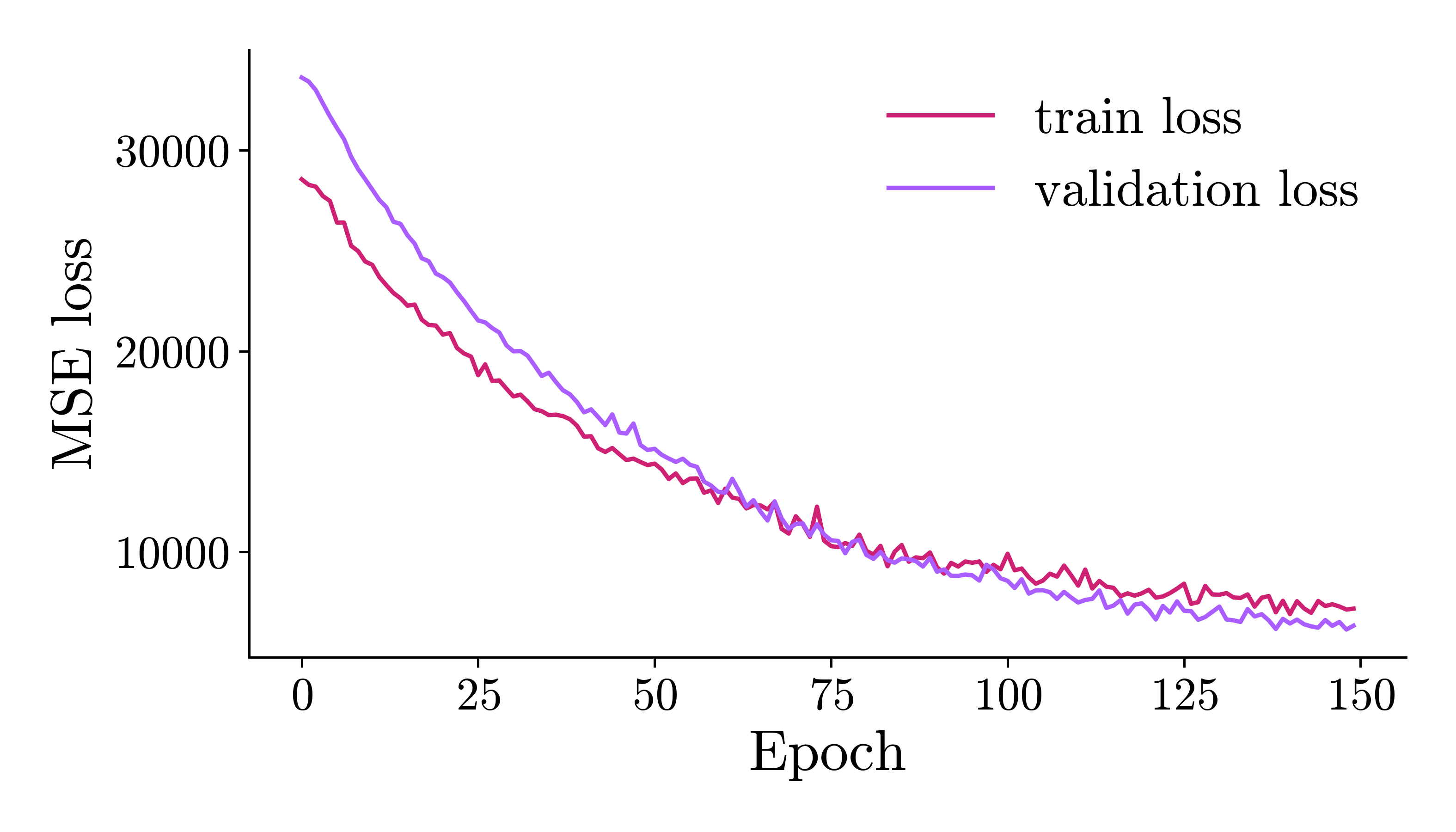
HQNR training | Epoch 1/150 | loss=28556.850369 | val_loss=33623.300781 | elapsed=2.9s | eta=433.1s
HQNR training | Epoch 2/150 | loss=28281.023980 | val_loss=33419.722656 | elapsed=5.6s | eta=411.2s
HQNR training | Epoch 3/150 | loss=28189.342122 | val_loss=32996.566406 | elapsed=8.3s | eta=408.6s
...
HQNR training | Epoch 149/150 | loss=7139.822401 | val_loss=6145.080078 | elapsed=399.1s | eta=2.7s
HQNR training | Epoch 150/150 | loss=7184.452705 | val_loss=6334.184277 | elapsed=401.1s | eta=0.0s
-0.44105827808380127
variational_type and basis are passed explicitly, and not left to their
defaults. All four arguments of the ansatz default to None, which means "use the
value of the layer that you named". Basic uses the "basic" variational block,
measured in the Z basis. This problem needs the stronger block. "strong" applies
the three rotations RZ, RY and RZ to each qubit in each layer, so it has three
times as many weights at the same depth, and it is what brings the loss down over
150 epochs. Without these two arguments, the same run ends near 13600 instead of
7180.
This example shows how to use the library, not a competitive model
The score above is negative. This means that the regressor does worse on the
held-out split than a prediction of the training mean would. A Ridge
baseline on the same split reaches about 0.42. The curve below does go down,
and that is what the example is for, but it stops far short of a useful model.
After 150 epochs, the loss has not reached the variance of the target. The
target ranges from 25 to 346, and this whole range comes from the linear
head alone, on top of a quantum layer whose outputs are in [-1, 1]. Scale the
target before you draw any conclusion from the score.
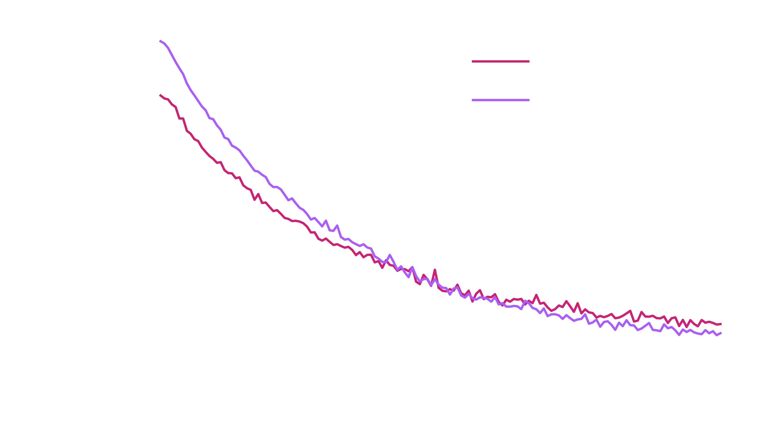
Inspect the training curve. The plot is drawn twice, once for each theme, so that
the site can show the one that matches the theme of the reader. rc_params("dark")
makes the backgrounds of the figure, the axes and the legend transparent, and turns
the text white. Everything else is the same in the two figures:
import matplotlib
import matplotlib.pyplot as plt
from eigenkit.datasets import STYLE_COLORS, rc_params

for theme in ("light", "dark"):
    with matplotlib.rc_context(rc_params(theme=theme)):
        fig, ax = plt.subplots(figsize=(7, 4))
        ax.plot(model.train_losses_, color=STYLE_COLORS[0], label="train loss")
        ax.plot(model.validation_losses_, color=STYLE_COLORS[1], label="validation loss")
        ax.set_xlabel("Epoch")
        ax.set_ylabel("MSE loss")
        ax.legend()
        fig.tight_layout()
        fig.savefig(f"hqnr_training_curve_{theme}.png")
        if theme == "light":
            plt.show()
        else:
            plt.close(fig)
You can choose the loss with loss_func ("mse", "mae" or "huber").
QSVR
QSVR is the quantum support vector regressor. It works like QSVC, but for
regression:
from eigenkit import QSVR

model = QSVR(feature_map="Angle", reps=1, C=1.0, epsilon=0.1)
model.fit(X_train, y_train)
print(model.score(X_test, y_test))
Time-series forecasting
QuantumTimeSeriesRegressor wraps an inner estimator with a sliding window. Here
the inner model is RecurrentHQNR, so each window is read as a sequence, and it is
not flattened first.
import numpy as np
from eigenkit import (
    RecurrentHQNR,
    QuantumTimeSeriesRegressor,
)

# Toy sine wave with a 1-D feature axis.
t = np.linspace(0, 8 * np.pi, 100).astype(np.float32)
series = np.sin(t).reshape(-1, 1)  # (100, 1)
target = np.sin(t + 0.1).astype(np.float32)

inner = RecurrentHQNR(
    seq_feature_dim=1,
    rnn_type="gru",
    rnn_hidden_dim=4,
    depth=1,
    variational_type="strong",
    basis="Y",
    epochs=50,
)

model = QuantumTimeSeriesRegressor(
    estimator=inner,
    in_size=10,
    shift=1,
)
model.fit(series, target)
predictions = model.predict(series)

# The wrapper carries the inner estimator's loss history.
history = model.train_losses_
print(f"epochs: {len(history)}   first: {history[0]:.6f}   last: {history[-1]:.6f}")

# score() windows and aligns the targets the same way predict does.
for name, value in model.score(series, target, return_dict=True).items():
    print(f"{name:5s} {value: .6f}")
RecurrentHQNR training | Epoch 1/50 | loss=0.561485 | elapsed=0.1s | eta=2.5s
RecurrentHQNR training | Epoch 2/50 | loss=0.533511 | elapsed=0.1s | eta=2.3s
RecurrentHQNR training | Epoch 3/50 | loss=0.497451 | elapsed=0.1s | eta=2.3s
...
RecurrentHQNR training | Epoch 49/50 | loss=0.002330 | elapsed=2.4s | eta=0.0s
RecurrentHQNR training | Epoch 50/50 | loss=0.003000 | elapsed=2.4s | eta=0.0s
epochs: 50   first: 0.561485   last: 0.003000
r2     0.993713
mse    0.003008
mae    0.040461
rmse   0.054849
mape   0.293061
variational_type and basis are set here for the same reason as for HQNR
above. The arguments of the ansatz default to those of the layer, and this problem
needs the "strong" block. Without these two arguments, the same run ends at an
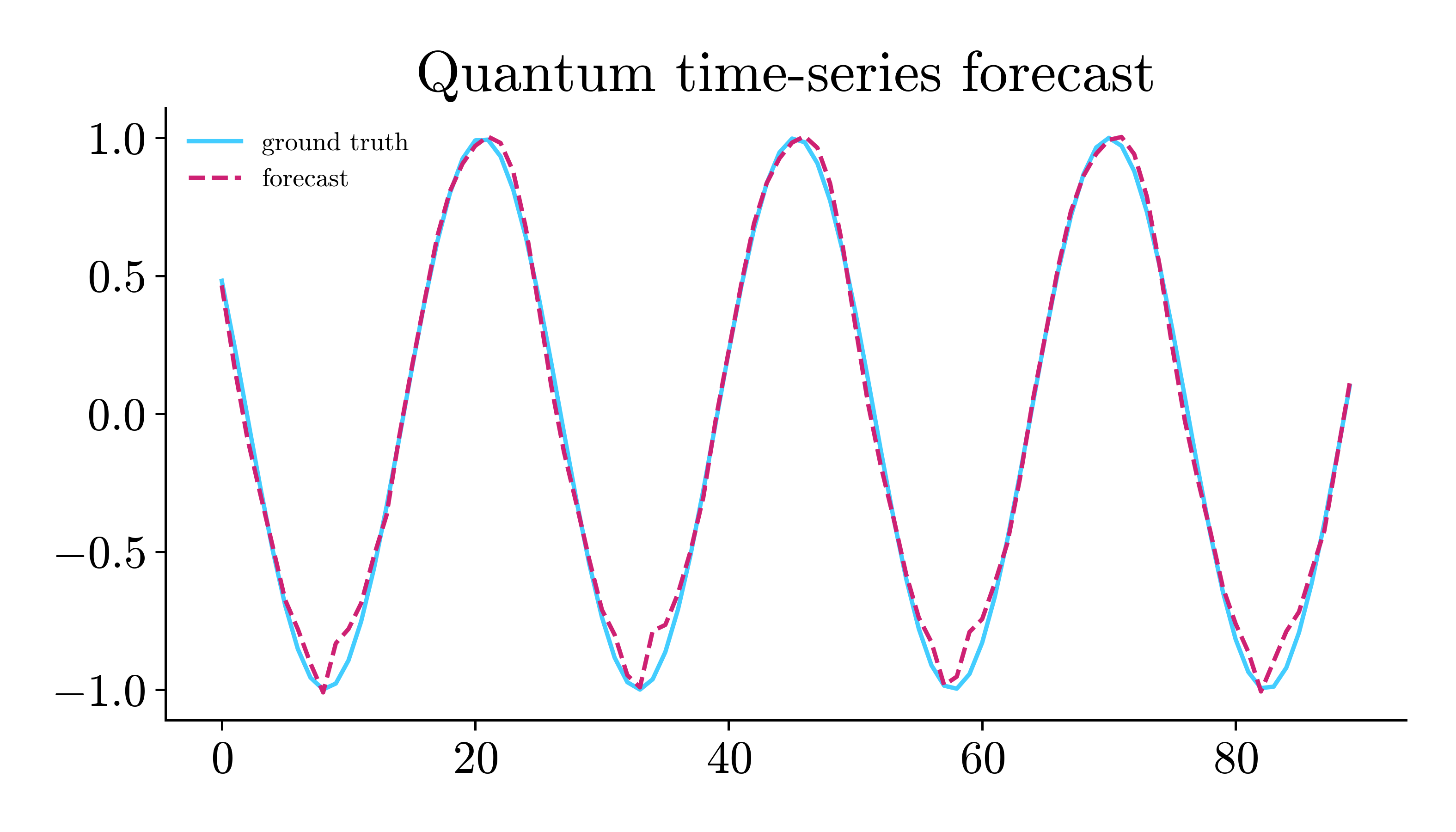
R² of 0.9087 and an rmse of 0.209, instead of the 0.9937 and 0.055 above.
That forecast overshoots 1.0 and lags on every descent.
By default, score() returns only the R², which is what cross_val_score and
GridSearchCV expect. return_dict=True gives the five figures above. Read mape
(the mean absolute percentage error) with care on this target. A sine crosses zero,
so a percentage error is large wherever the true value is near zero. So 0.29 says
less about the fit than the rmse (the root mean squared error) of 0.055 does, for
a signal of amplitude 1. model.train_losses_ holds the loss of every epoch, if
you want to plot it next to the forecast.
Visualising the forecast
import matplotlib
import matplotlib.pyplot as plt
from eigenkit.datasets import STYLE_COLORS, rc_params

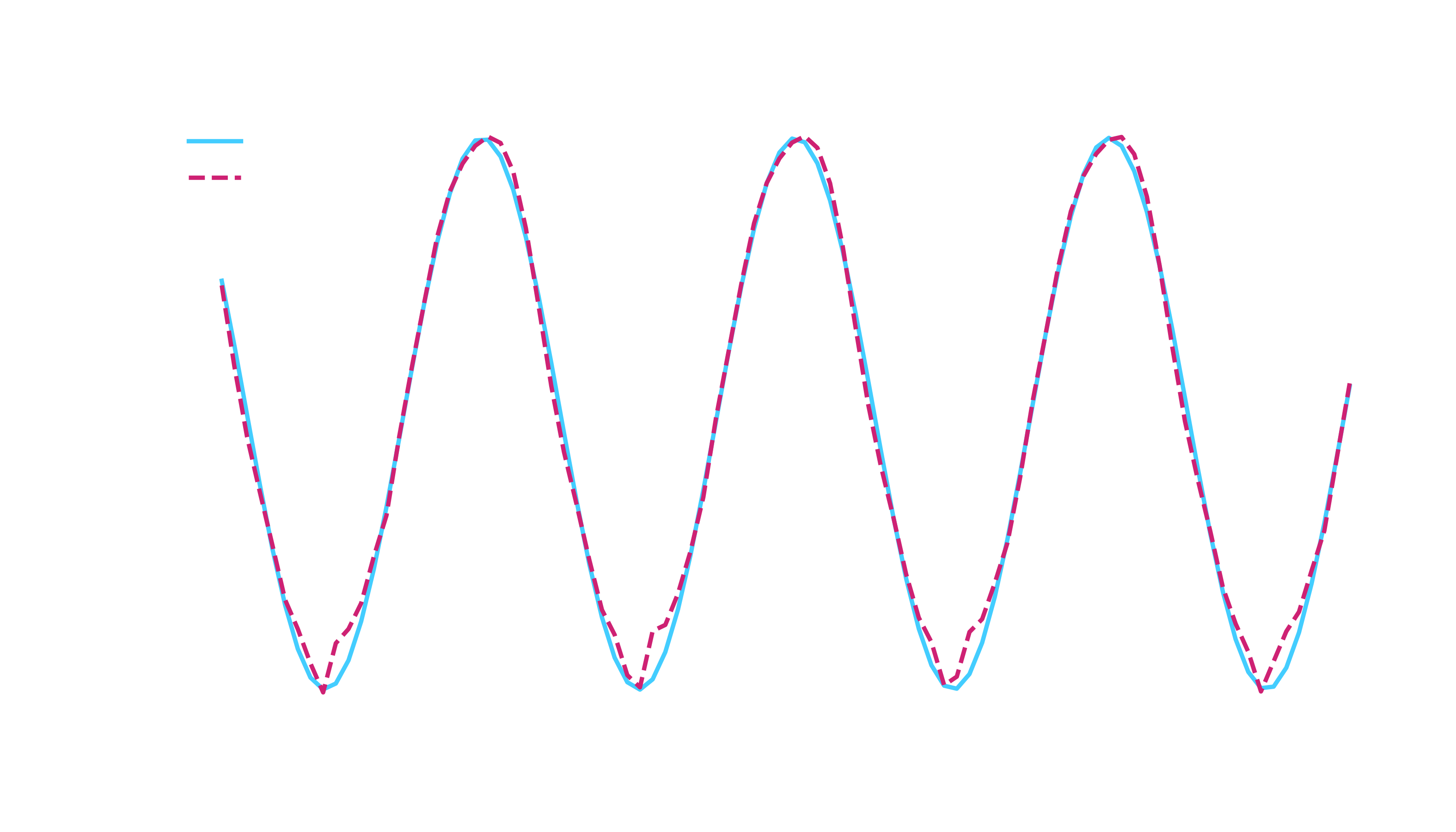
# QuantumTimeSeriesRegressor predicts targets at indices
# `i + in_size - 1 + shift`, so we align ground truth with that range.
aligned = target[10:]  # in_size=10, shift=1

for theme in ("light", "dark"):
    with matplotlib.rc_context(rc_params(theme=theme)):
        fig, ax = plt.subplots(figsize=(7, 4))
        ax.plot(aligned, color=STYLE_COLORS[3], label="ground truth")
        ax.plot(predictions, color=STYLE_COLORS[0], label="forecast", linestyle="--")
        ax.legend(fontsize=9, loc="upper left")
        ax.set_title("Quantum time-series forecast")
        fig.tight_layout()
        fig.savefig(f"quantum_timeseries_forecast_{theme}.png")
        if theme == "light":
            plt.show()
        else:
            plt.close(fig)
Swapping the inner estimator
Any compatible regressor can be the inner estimator. For tabular estimators (such
as HQNR and QSVR), the wrapper flattens each window before fit and
predict:
from eigenkit import HQNR, QuantumTimeSeriesRegressor

# in_size * n_features = 10 * 1 = 10 features per flattened window.
inner = HQNR(in_features=10, depth=2, epochs=20)
model = QuantumTimeSeriesRegressor(estimator=inner, in_size=10, shift=1)
model.fit(series, target)
predictions = model.predict(series)