Hybrid Classical-Quantum Model

This example places an Ensemble layer inside a classical nn.Sequential pipeline, and trains the pipeline on the moons dataset.

Data preparation

import torch
from sklearn.datasets import make_moons
from sklearn.model_selection import train_test_split
from sklearn.preprocessing import StandardScaler

X, y = make_moons(n_samples=1000, noise=0.2, random_state=42)
X_train, X_test, y_train, y_test = train_test_split(
    X,
    y,
    test_size=0.2,
    random_state=42,
)

scaler = StandardScaler()
X_train = scaler.fit_transform(X_train)
X_test = scaler.transform(X_test)

X_train_t = torch.tensor(X_train, dtype=torch.float32)
y_train_t = torch.tensor(y_train, dtype=torch.long)
X_test_t = torch.tensor(X_test, dtype=torch.float32)
y_test_t = torch.tensor(y_test, dtype=torch.long)

Model definition

The quantum layer is Ensemble, placed between two classical linear layers. The first linear layer maps the two features of the moons data to an input with more dimensions, which the quantum circuit can use.

import torch
from torch import nn
from eigenkit import Ensemble


class HybridModel(nn.Module):
    def __init__(self, hidden_size: int, n_qubits: int, depth: int):
        super().__init__()
        self.layers = nn.Sequential(
            nn.Linear(2, hidden_size),
            nn.ReLU(),
            Ensemble(
                in_features=hidden_size,
                n_qubits=n_qubits,
                depth=depth,
            ),
            nn.ReLU(),
            nn.Linear(hidden_size, 2),
        )

    def forward(self, x: torch.Tensor) -> torch.Tensor:
        return self.layers(x)

hidden_size must be divisible by n_qubits, because Ensemble splits its input into chunks of size n_qubits and runs one independent circuit on each chunk. The outputs of the circuits are concatenated, so the layer returns hidden_size values.

Training loop

from torch import optim
from torch.utils.data import TensorDataset, DataLoader


def train(
    model,
    X_train,
    y_train,
    X_test,
    y_test,
    loss_fn,
    optimizer,
    num_epochs=10,
    batch_size=32,
):
    loader = DataLoader(
        TensorDataset(X_train, y_train),
        batch_size=batch_size,
        shuffle=True,
    )

    for epoch in range(num_epochs):
        model.train()
        running_loss = 0.0
        for xb, yb in loader:
            preds = model(xb)
            loss = loss_fn(preds, yb)
            optimizer.zero_grad()
            loss.backward()
            optimizer.step()
            running_loss += loss.item() * xb.size(0)

        model.eval()
        with torch.no_grad():
            acc = (model(X_test).argmax(1) == y_test).float().mean().item()
        print(
            f"Epoch {epoch + 1}/{num_epochs} | "
            f"loss: {running_loss / len(X_train):.4f} | "
            f"test_acc: {acc:.4f}"
        )

Run training

torch.manual_seed(42)

model = HybridModel(hidden_size=12, n_qubits=4, depth=2)
loss_fn = nn.CrossEntropyLoss()
optimizer = optim.Adam(model.parameters(), lr=0.005)

train(
    model,
    X_train_t,
    y_train_t,
    X_test_t,
    y_test_t,
    loss_fn,
    optimizer,
    num_epochs=15,
    batch_size=32,
)

Epoch 1/15 | loss: 0.6283 | test_acc: 0.8200
...
Epoch 15/15 | loss: 0.1134 | test_acc: 0.9850

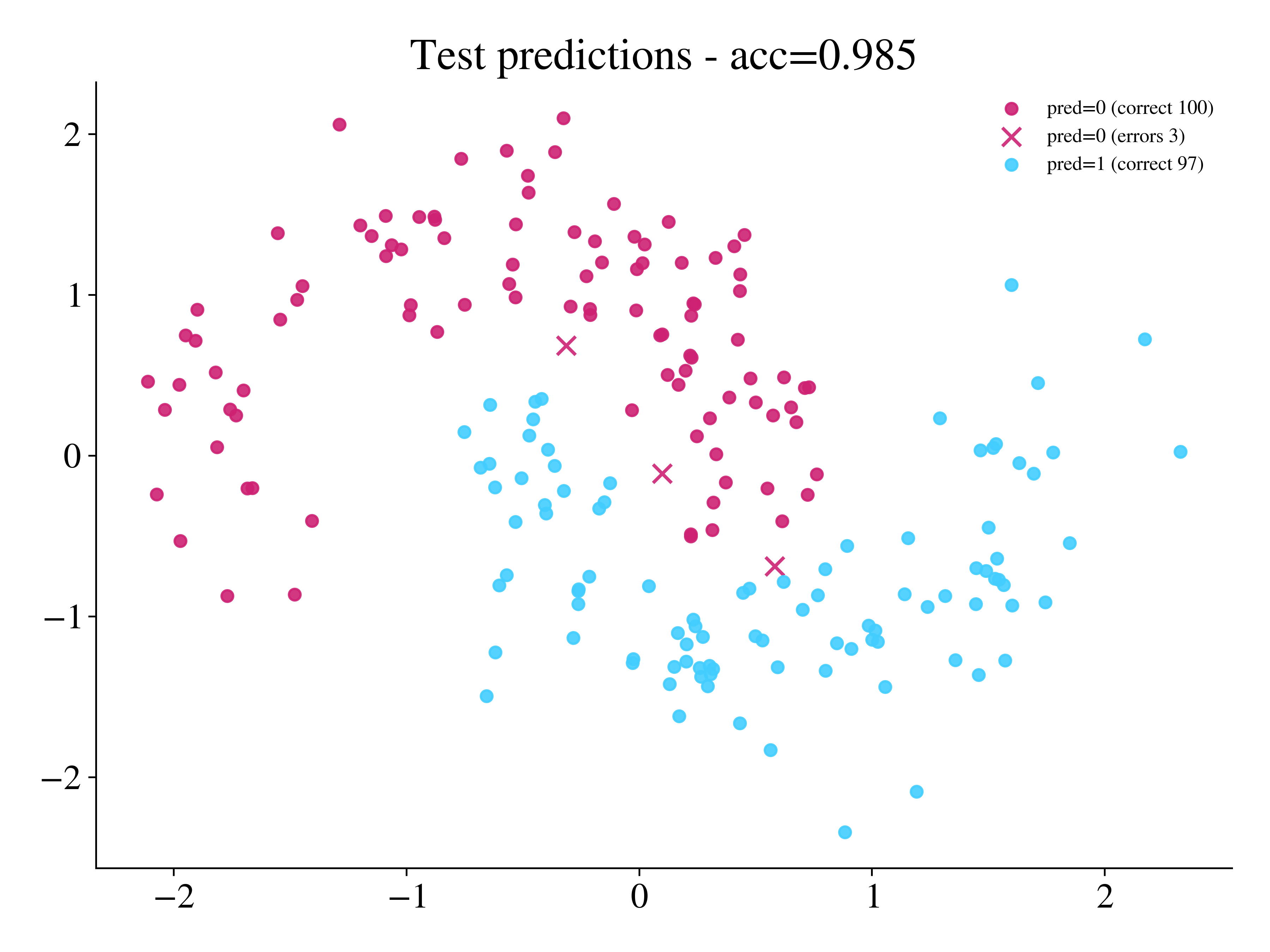
Visualise predictions

import matplotlib.pyplot as plt
import matplotlib
from matplotlib.colors import ListedColormap
from eigenkit.datasets import STYLE_COLORS, rc_params


def plot_predictions(model, X_test, y_test):
    model.eval()
    with torch.no_grad():
        pred = model(X_test).argmax(1)
    acc = (pred == y_test).float().mean().item()
    correct = pred.eq(y_test)
    class_cmap = ListedColormap([STYLE_COLORS[0], STYLE_COLORS[3], STYLE_COLORS[5]])

    with matplotlib.rc_context(rc_params(theme="light")):
        plt.figure(figsize=(8, 6))
        for cls in torch.unique(pred).tolist():
            color = class_cmap(int(cls) % class_cmap.N)
            mask = pred.eq(cls)
            plt.scatter(
                X_test[mask & correct, 0],
                X_test[mask & correct, 1],
                s=28,
                marker="o",
                alpha=0.9,
                label=f"pred={cls} (correct {int((mask & correct).sum())})",
                color=color,
            )
            if (mask & ~correct).any():
                plt.scatter(
                    X_test[mask & ~correct, 0],
                    X_test[mask & ~correct, 1],
                    s=70,
                    marker="x",
                    alpha=0.9,
                    label=f"pred={cls} (errors {int((mask & ~correct).sum())})",
                    color=color,
                )
        plt.title(f"Test predictions - acc={acc:.3f}")
        plt.legend(fontsize=9)
        plt.tight_layout()
        plt.show()


plot_predictions(model, X_test_t, y_test_t)

The predictions of the hybrid model on the moons test data (light theme).

See the Layers guide for the full application programming interface (API).