Algorithms

eigenkit.algorithms contains three standalone quantum algorithms. HHL solves linear systems with the algorithm of Harrow, Hassidim and Lloyd (HHL). IQAE runs Iterative Quantum Amplitude Estimation (IQAE). PortfolioRiskEstimator estimates portfolio risk and is built on IQAE. The first two are single-call solvers. You configure a solver in its constructor, call one method, and get back a frozen result dataclass. There is no fit/predict cycle and no fitted state to keep. PortfolioRiskEstimator works differently, because it is first fitted to a price history (see below).

All three default to provider="numpy", the built-in simulator that every installation includes. Two of the modes of IQAE, a callable oracle and shot_mode="provider", need provider="pennylane" and the pennylane extra. The API reference at the end of this page lists the full signatures and defaults, with notes on every argument.

Solver	Answers	Result carries
`HHL`	the solution `x` of `Ax = b`	`solution`, `euclidean_norm`, `residual`, `success_probability`, `readout_probability`, `raw_solution`
`IQAE`	an unknown amplitude, with an interval	`estimation`, `confidence_interval`, `n_rounds`, `n_oracle_calls`
`PortfolioRiskEstimator`	the Value at Risk (VaR) and the Conditional Value at Risk (CVaR)	`var`, `cvar`, `tail_probability`, `confidence_interval`, `iqae_result`

Each result is a frozen dataclass, so its fields can be read but not changed.

The theory behind these two algorithms is explained in the HHL and IQAE chapters of the Algorithms Explained section.

What counts as a solver

A solver inherits from BaseQuantumSolver. It has a solve() method that takes a problem and returns a result, with no training phase and no fitted state. Four classes are solvers: HHL and IQAE on this page, the Quantum Approximate Optimization Algorithm (QAOA) in optimization, and the Variational Quantum Eigensolver (VQE) in chemistry. The base class is defined in core and not in algorithms, because QAOA and VQE depend only on core.

from eigenkit.core import BaseQuantumSolver
from eigenkit import HHL

isinstance(HHL(), BaseQuantumSolver)  # True

solve() is an abstract method, so a solver class that does not implement it cannot be instantiated. The base class also stores the provider attribute for all four solvers. Each subclass sets its own default in its signature and passes it to the base class, and the default is "numpy" for all four.

PortfolioRiskEstimator does not inherit from BaseQuantumSolver, by design. It follows the scikit-learn estimator pattern, with fit(), estimate() and var_at() and no solve() method, so isinstance returns False for it. This is the expected result when you check whether an object can be given a problem directly.

HHL: Linear systems

HHL solves Ax = b. If A is Hermitian, it is used directly, even when it is not positive semidefinite. Any other invertible square matrix is converted to the normal equations A†Ax = A†b, which have the same solution and a Hermitian system matrix.

import numpy as np
from eigenkit import HHL

A = np.array([[1.0, 0.5], [0.5, 1.5]])
b = np.array([1.0, 0.0])

result = HHL(n_eigenvalue_qubits=3, provider="numpy").solve(A, b)

print(result.solution.real)  # [ 1.1888 -0.3789]
print(np.linalg.solve(A, b))  # [ 1.2    -0.4   ]  the classical answer
print(result.residual)  # 0.026
print(result.success_probability)  # 0.7282

The solution is returned as a complex array because it is read from a statevector. Use .real when the system is real.

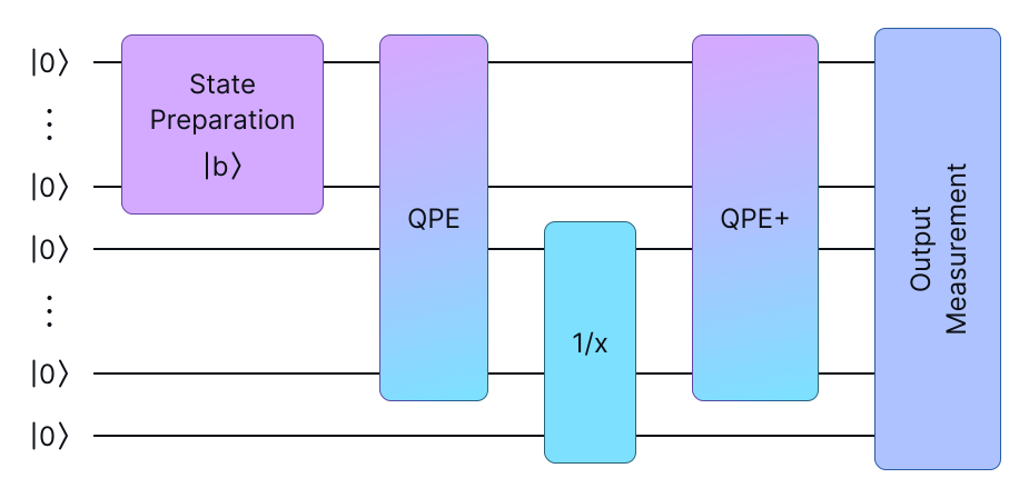
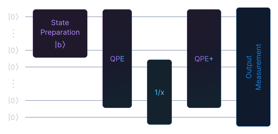
The circuit HHL builds (light theme) The circuit HHL builds (dark theme)

The circuit that solve() builds has the same stages in both modes. |b⟩ is prepared on the input register. Phase estimation writes the eigenvalues of A into the clock register, whose size is set by n_eigenvalue_qubits. The 1/x rotation turns each eigenvalue into its reciprocal on the ancilla, and QPE+, the adjoint of quantum phase estimation (QPE), resets the clock register. The mode argument changes how the phase-estimation step is built, but not these stages. The answer is read from the branch where the ancilla is in the useful state and the clock register has returned to zero. This is why the backend must provide a statevector, and readout_probability measures the weight of that branch. success_probability counts only the ancilla, over every clock state.

Two arguments control the accuracy. n_eigenvalue_qubits sets the size of the clock register, which determines how finely the spectrum is resolved. A finer resolution needs a larger circuit. The example above uses 3 qubits and gets within about 1 % of the classical answer. epsilon is an eigenvalue cutoff. Eigenvalues below it are treated as noise and dropped, which prevents a nearly singular system from producing very large values. The evolution time t is chosen automatically from the spectrum, and we recommend keeping the automatic value. If t is too large, phase estimation aliases. The solver detects this and reports it, instead of returning a wrong answer.

A third argument, mode, chooses which circuit is built. The default, mode="reference", computes the eigenvalues classically and applies e^{iAt} as one dense unitary. It is exact and fast, but its cost does not reflect how HHL scales. mode="honest" builds the same algorithm from elementary gates instead. The evolution is Trotterised from the Pauli decomposition of A, and the evolution time comes from a Gershgorin bound, so no circuit parameter depends on an eigendecomposition. This mode needs at least two clock qubits, and trotter_steps ("auto" by default), trotter_order and trotter_tolerance control the Trotter grid. The HHL page compares the two modes, and the worked example measures the cost of each one.

The result has six fields. residual is the best measure of the quality of a run. It is the relative error ‖Ax − b‖ / ‖b‖, computed against the original system, so it measures the answer itself and not the algorithm's own estimate of it. success_probability matters for anything beyond a simulator. It is the probability that the ancilla lands in the useful branch, so its reciprocal is roughly the number of times a real device would have to repeat the state preparation. readout_probability is the narrower physical rate: the probability that both the ancilla and the clock register land where the solution is read, which is what an estimate from shots needs. raw_solution holds the post-selected amplitudes produced by the circuit, before the classical rescaling. It is the only part of the output that comes directly from the quantum computation.

The circuit reads the full statevector and post-selects, so the backend must provide a statevector. The numpy simulator, PennyLane default.qubit and lightning.qubit, and Qiskit Aer all do. Shot-based backends and quantum processing units (QPUs) raise NotImplementedError.

IQAE: Amplitude estimation

IQAE estimates a = |⟨ψ₁|A|0⟩|², the probability that a state-preparation circuit ends in the marked state. The estimate comes with a confidence interval, so you do not have to infer one from repeated runs.

The oracle is the state preparation A itself. It can be given as a CircuitSpec built with CircuitBuilder, or as a PennyLane callable oracle(wires), which needs provider="pennylane". The last qubit is the ancilla. The oracle must have no trainable weights and no inputs, and its number of qubits must equal n_qubits.

import numpy as np
from eigenkit import CircuitBuilder
from eigenkit import IQAE

# RY(pi/3) on the ancilla prepares an amplitude of sin^2(pi/6) = 0.25 exactly.
qc = CircuitBuilder(n_qubits=2)
qc.ry(np.pi / 3, qubit=1)
oracle = qc.build()

result = IQAE(epsilon=0.02, alpha=0.05, n_qubits=2, random_state=0).solve(oracle)

print(result.estimation)  # 0.246
print(result.confidence_interval)  # (0.2407, 0.2513)  contains the true 0.25
print(result.n_rounds)  # 4
print(result.n_oracle_calls)  # 2600

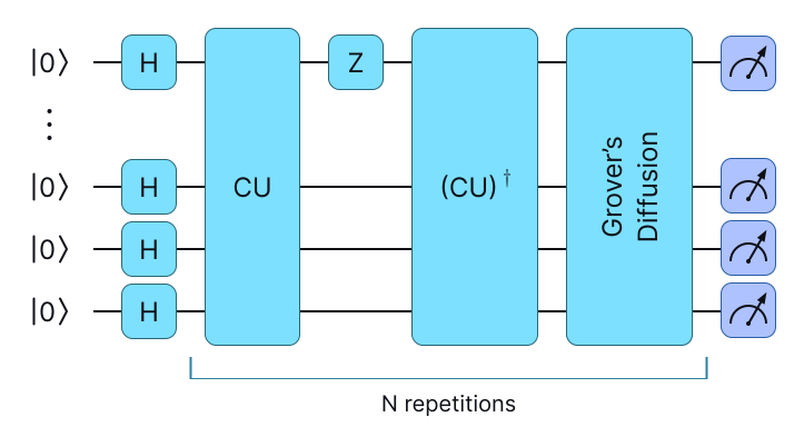
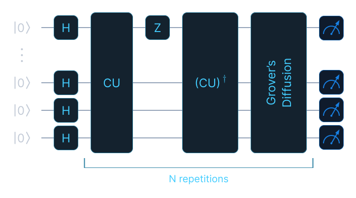
The Grover operator amplitude estimation iterates (light theme)

This is the operator that IQAE repeats. One repetition applies the state preparation A (the oracle you pass, drawn as CU in the figure), then a phase flip on the marked state, then A†, then the diffusion operator. Each repetition rotates more amplitude onto the marked state. The adaptive rule of Grinko et al. decides how the number of repetitions grows from one round to the next, and n_oracle_calls counts the applications of A and A† over the whole run. The Hadamard layer at the start comes from Grover search, where A prepares the uniform superposition. In IQAE, the initial state is whatever your oracle prepares.

epsilon, alpha and n_qubits are required and have no default values. epsilon is the half-width of the interval that you are willing to accept, alpha is the probability that the interval is allowed to miss the true value, and n_qubits is the number of qubits of the oracle, including the ancilla.

Set random_state whenever a run must be repeatable, because the shot noise is seeded from it.

The result contains the estimate, its interval, and two cost counters. Use n_oracle_calls when comparing against classical sampling, because the advantage of the algorithm is its convergence rate: as epsilon gets smaller, the error decreases roughly as 1/n_oracle_calls, compared with 1/√n when drawing n classical samples.

PortfolioRiskEstimator: VaR and CVaR

PortfolioRiskEstimator takes a price history, fits a loss distribution to it, and reports the Value at Risk (VaR) and the Conditional Value at Risk (CVaR). The tail probability behind these numbers is estimated with IQAE, which is the quantum part of the method. By default, VaR and CVaR are computed classically from the fitted bins. A quantum bisection, described below, is optional.

Not financial advice

The estimates come from a model fitted to the price history you pass in, and they carry no guarantee. They are not investment advice, and they are not meant to be the only basis of a decision about risk.

fit takes X of shape (n_timesteps, n_assets), containing closing prices and not returns. Portfolio weights are optional, and all assets are weighted equally by default.

import numpy as np
from eigenkit import PortfolioRiskEstimator

rng = np.random.default_rng(0)
returns = rng.normal(0.0005, 0.02, size=(250, 3))
prices = 100 * np.exp(np.cumsum(returns, axis=0))

estimator = PortfolioRiskEstimator(n_qubits=5, provider="numpy", random_state=0)
estimator.fit(prices, weights=np.array([0.5, 0.3, 0.2]))

risk = estimator.estimate(confidence_level=0.95)

print(risk.var)  # 0.0237   loses at most 2.37% on 95% of days
print(risk.cvar)  # 0.0262   average loss on the worst 5%
print(risk.tail_probability)  # 0.0659   IQAE estimate of the tail mass

n_qubits sets the resolution. One qubit is the ancilla and the others discretise the loss distribution, so 5 qubits give 16 bins. With coarse bins, the VaR changes in visible steps. If the result looks like a round number, increase n_qubits first.

Two arguments decide how much of the computation is quantum. With the default n_bisection_steps=0, VaR and CVaR are the classical values from the bins, and only the tail probability is estimated on the circuit. A positive value runs a binary search that calls IQAE at every step to find the VaR threshold. measure_tail_probability controls the final IQAE call. Turn it off when you only need the classical values and do not want to run the circuit at all.

The result reports var and cvar as fractions of the portfolio value, with the estimated tail_probability and a confidence interval for it. The interval applies to the tail probability, not to the VaR. The nested iqae_result contains the underlying IQAE estimate, and is None when the final IQAE call was skipped.

var_at() is the array version of estimate(). It takes a list of confidence levels and returns the VaR at each one. For the fit above, var_at([0.90, 0.95, 0.99]) returns [0.0144, 0.0237, 0.0330], and the middle value matches estimate(0.95).var.

The method is not called predict(), on purpose. In scikit-learn, predict takes samples from the same feature space that fit received, and this method takes confidence levels instead. Calling predict() raises an error that points to var_at().

A confidence level below 0.5 is valid (the VaR at 0.5 is the median loss), but such values also look like a series of returns or normalised features, so var_at() issues a warning in that case. Passing such an array is the only mistake that this method does not reject with an error. A price series is rejected because prices are not in (0, 1), and a price matrix is rejected because it is not 1-D.

API reference

`eigenkit.algorithms`

General-purpose quantum algorithms.

This package contains three algorithms:

HHL solves linear systems with the algorithm of Harrow, Hassidim and Lloyd (HHL).
IQAE runs Iterative Quantum Amplitude Estimation (IQAE).
PortfolioRiskEstimator estimates the Value at Risk (VaR) and the Conditional Value at Risk (CVaR) of a portfolio with IQAE.

HHL and IQAE inherit from BaseQuantumSolver, the base class for solvers that work in a single call and keep no fitted state. The Quantum Approximate Optimization Algorithm (QAOA) and the Variational Quantum Eigensolver (VQE) also inherit from it, in their own packages. The base class is defined in core because QAOA and VQE depend only on core. PortfolioRiskEstimator does not inherit from it, by design. It is a scikit-learn-style estimator, registered in the estimator registry of eigenkit.qml so that it can be saved and loaded. It therefore needs scikit-learn and is imported on first use; HHL and IQAE need only the core install.

`HHL`

Bases: BaseQuantumSolver

Quantum linear solver based on the algorithm of Harrow, Hassidim and Lloyd (HHL).

Solves Ax = b for any invertible square matrix A. If A is Hermitian, it is used directly, even when it is not positive semidefinite. Any other matrix is converted to the normal equations A†Ax = A†b, which have the same solution and a Hermitian, positive semidefinite system matrix. The cost of this conversion is that the condition number κ is squared.

The circuit itself inverts the eigenvalues. It applies controlled RY rotations to the ancilla, with one fixed angle for each state of the clock register, so the reciprocal 1/λ of each eigenvalue is encoded in the amplitudes without any classical division by the eigenvalues. The readout is different: it uses the simulator's full statevector and keeps only the part where the ancilla is in |1⟩ and the clock register is in |0⟩. HHL produces the quantum state |x⟩, so reading a classical vector from it is only possible on a simulator. See HHLResult.

Warning

The backend must provide statevector() on its compiled circuit. The built-in numpy simulator, PennyLane default.qubit and lightning.qubit, and Qiskit Aer all do. A custom backend registered with register() must implement it, otherwise solve() raises NotImplementedError.

Scope and scaling. HHL is efficient only when three conditions hold: A is a sum of a few short Pauli terms, A is well conditioned, and the state |b⟩ can be prepared efficiently.

Hamiltonian simulation. e^{iAt} is Trotterised from the Pauli decomposition of A, so its cost follows the number of Pauli terms. This means sparsity in the Pauli basis, which is different from sparsity of the matrix. The module algorithms/_hamiltonian_sim.py explains what this means in practice. In short, a sparse matrix is not necessarily cheap to simulate here.
State preparation. |b⟩ is prepared with AmplitudeEncoding, which is treated as an oracle of unit cost. Loading general amplitudes costs O(N) gates, so a real speedup assumes that b comes from a formula, from an earlier quantum routine, or from a quantum random-access memory (qRAM).
Conditioning. The condition number κ is never an input. It only bounds the achievable success probability and the size of the clock register.
Inversion angles. The gates are elementary (see _uniformly_controlled_ry()), so the circuit built in "honest" mode contains no unitary-matrix gate. However, the 2^n_l angles, where n_l is the number of clock qubits, are listed one by one instead of being computed by the circuit. The classical description of the circuit therefore has size Θ(2^n_l). The circuit can be built from elementary gates, but its description is not compact.

Solvers for dense matrices, for example the one of Wossnig, Zhao and Prakash, reach a quadratic speedup when the spectral norm is bounded. They need a specialised memory architecture that this package does not provide.

Real and complex inputs. For real A and b, the readout discards the imaginary part. The leading error of the Trotter eigenvectors enters the raw vector as a purely imaginary component, so discarding the imaginary part removes it. This matters at trotter_order=1, where it improves the convergence by one order: the measured error falls as steps⁻² for real inputs, and as steps⁻¹ for a complex Hermitian A or a complex b, which keep that error. At trotter_order=2, the default, the first-order commutator already cancels by construction, so there is nothing left to remove, and real and complex inputs both converge as steps⁻². This advantage was not designed. It depends on the test for real inputs in solve(), so a change to that test changes the convergence rate at order 1.

Parameters:

Name	Type	Description	Default
`n_eigenvalue_qubits`	`int`	The number of qubits in the clock register. Eigenvalues are resolved into `2**n_eigenvalue_qubits` buckets. The value must be at least 1, and at least 2 in `"honest"` mode. More qubits give a finer resolution of the spectrum and a larger circuit. The default is `4`.	`4`
`t`	`float \| None`	The evolution time for `U = e^{iAt}`. If given, it must be positive and finite. If `None`, it is chosen automatically: from the spectrum in `"reference"` mode, and from a Gershgorin bound in `"honest"` mode. The default is `None`.	`None`
`epsilon`	`float`	The relative eigenvalue cutoff, in `[0, 1)`. For a Hermitian `A`, buckets whose estimated eigenvalue is below `epsilon * λ_max` are treated as zero. For the normal equations, the cutoff applies to the singular values instead, and it is implemented as `epsilon²` on the squared spectrum. If no eigenvalue is above the cutoff, `solve()` raises an error. The default is `0.01`.	`0.01`
`provider`	`ProviderSpec`	The backend to use: a registered name (`"numpy"`, `"pennylane"`, `"qiskit"` and so on), a config instance, or a backend object. It must provide `statevector()`. The default is `"numpy"`.	`'numpy'`
`mode`	`str`	How the circuit is built. This argument is keyword-only. `"reference"` (the default): the eigenvalues are computed classically with `eigvalsh`, `e^{iAt}` is a dense `QubitUnitary` computed with `expm`, and `t` is tuned to the known spectrum. This mode is fast and exact, but the `O(N³)` precomputation and the dense unitary mean that its cost does not follow the scaling of HHL. `"honest"`: the circuit is built as it would be on hardware. No eigendecomposition sets any circuit parameter: `t` comes from a Gershgorin bound, the scaling constant `C` of the inversion comes from the resolution of the clock register (see `_honest_qpe_params()`), and `e^{iAt}` is Trotterised into elementary gates. This mode requires `n_eigenvalue_qubits >= 2`. Input validation still runs an `O(N³)` rank check. This check makes the solver safer to use and is not part of the algorithm; see `solve()`.	`'reference'`
`trotter_steps`	`int \| Literal['auto']`	The number of Trotter steps for the base evolution time in `"honest"` mode. It is ignored in `"reference"` mode. With `"auto"`, the default, the solver picks the smallest number of steps for which a computable bound on the Trotter drift `‖A_eff − A‖` stays below `trotter_tolerance × C`, which is below the eigenvalue resolution of the clock register. This matters because, with a fixed step size, the circuit is exact HHL for an effective matrix `A_eff` whose eigenvectors are rotated even when its eigenvalues are exact. That changes the direction of the answer while every check based on the spectrum reports success. An integer turns off the automatic choice, and the solver warns if the drift bound then exceeds `C/2`. Above that value, an extreme eigenvalue can be captured by the Nyquist bucket or wrap around the branch cut. The automatic choice is limited by a gate budget, and the solver says so when the limit is reached. The default is `"auto"`.	`'auto'`
`trotter_order`	`int`	The Trotter order, 1 or 2. The default is `2`. The symmetric product of order 2 is a palindrome, so the first-order commutator cancels, the error falls from `O(τ)` to `O(τ²)`, and `A_eff` stays real for a real `A`. At order 1, `A_eff` picks up `Y`-type terms, and a real system returns a complex state. Order 1 is kept for cost comparisons.	`2`
`trotter_tolerance`	`float`	The target for `trotter_steps="auto"`. This argument is keyword-only. The drift bound must not exceed `trotter_tolerance × C`. The default, `0.25`, keeps the drift at a quarter of a bucket, below the `C/2` threshold at which the Nyquist bucket can capture an eigenvalue. At order 2, the cost grows as `steps ∝ 1/√tolerance`.	`_AUTO_TROTTER_TOLERANCE`

Raises:

Type	Description
`ValueError`	If `n_eigenvalue_qubits` is below 1, if `t` is not a positive finite number, or if `epsilon` is outside `[0, 1)`.

Example

This example solves a 2 × 2 Hermitian system:

import numpy as np
from eigenkit import HHL

A = np.array([[2, 1], [1, 2]], dtype=float)
b = np.array([1, 0], dtype=float)
result = HHL(n_eigenvalue_qubits=6).solve(A, b)
print(result.solution)
print(result.residual)

This example solves the same system on a faster simulator:

from eigenkit import HHL, PennyLaneConfig

solver = HHL(
    n_eigenvalue_qubits=6,
    provider=PennyLaneConfig(device_name="lightning.qubit"),
)
result = solver.solve(A, b)

`solve(A, b)`

Solve the linear system Ax = b.

Parameters:

Name	Type	Description	Default
`A`	`ndarray`	A real or complex square matrix, which must be invertible. A non-Hermitian matrix is converted to the normal equations.	required
`b`	`ndarray`	The right-hand side, of length `A.shape[0]`.	required

Returns:

Type	Description
`HHLResult`	An `HHLResult`. Its `solution` is read from the simulator's statevector and completed with a classical least-squares rescaling. See the notes on `HHLResult`.

Raises:

Type	Description
`ValueError`	If `A` is not square or is singular, if `b` has the wrong length, is zero or is not finite, or if `t` causes aliasing in quantum phase estimation (QPE).
`NotImplementedError`	If the backend does not implement `statevector()`, or if it returns something else, such as a density matrix.

Note

Validation runs one O(N³) singular value decomposition (SVD) to reject a singular A and to compute a condition number for the warnings. No quantity derived from it reaches t, C, the rotation angles or the number of Trotter steps, and changing it would leave the circuit exactly the same. mode="honest" therefore keeps its defining property, but solve() itself still does O(N³) work.

`HHLResult` `dataclass`

Bases: ValueEquality

Output of HHL.solve().

The result is read-only. Assigning to a field raises FrozenInstanceError, and writing into an array field raises ValueError. This prevents a mistyped = (instead of ==) or an in-place edit from leaving a result whose scalar fields describe a different run from the arrays it holds. To get a writable copy of an array, use np.array(result.field).

Results compare by value, including their arrays. They are not hashable, because a result is a collection of numbers and not a key, and a correct hash of a float array is expensive to compute.

Attributes:

Name	Type	Description
`solution`	`ndarray`	The best-fit `x` with `Ax ≈ b`. It is `float64` for real inputs, and `complex128` when `A` or `b` has a non-zero imaginary part.
`euclidean_norm`	`float`	The norm `‖solution‖` of the returned solution. It is computed after the classical least-squares rescaling, so it is not a norm that HHL itself measures.
`residual`	`float`	The relative error `‖Ax − b‖ / ‖b‖`, computed with the original `A` and `b`.
`success_probability`	`float`	The probability that the ancilla is in `\|1⟩`, summed over all states of the clock register.
`readout_probability`	`float`	The probability of the joint event from which the solution is read: the ancilla in `\|1⟩` and the clock register in `\|0…0⟩`. This is the physical post-selection rate. It is never larger than `success_probability`, so use it to estimate the number of shots.
`raw_solution`	`ndarray \| None`	The post-selected amplitudes as the circuit produced them. They are complex, and they come before the imaginary part is dropped and before the rescaling, so this is the only part of the output that comes directly from the quantum computation. The vector has unit norm, except when the size of the system is not a power of two. In that case it is a slice of a unit-norm state, and the Trotterised evolution leaks a small amount of weight into the zero padding.

Note

HHL produces the quantum state |x⟩, not a vector of numbers. The full array in this result is read from the simulator's statevector, which only a simulator can provide. On hardware, only expectation values can be measured, and extracting all N components of |x⟩ costs O(N) measurements, which cancels the speedup. In practice, |x⟩ is passed to another quantum routine, or used to estimate one observable. Recovering the sign of 1/λ needs a separate protocol. All of this applies to both values of mode.

Warning

solution is completed by two classical steps that hardware cannot perform. For real inputs, the imaginary part is discarded. The magnitude and the sign then come from a least-squares projection, x = raw · ⟨A·raw, b⟩ / ‖A·raw‖², which uses the full classical A and b. Only the direction of raw comes from the quantum computation. The rescaling can change residual by an order of magnitude, and for an indefinite A its sign correction is not reliable, because ⟨Ax, b⟩ ≥ 0 does not imply ⟨x, A⁻¹b⟩ ≥ 0.

`__post_init__()`

Make the array fields read-only.

Freezing the dataclass prevents a field from being reassigned, but it does not prevent writing into the array that the field holds, and a result that has been written into still reports the scalar values of the original run. The result therefore keeps its own copy, so the array it was built from can still be changed by the caller. To get a writable copy, use np.array(result.solution).

Both array fields are frozen. raw_solution is optional, and freeze_arrays would turn a None into a zero-dimensional object array, so it is only frozen when the run recorded one.

`IQAE`

Bases: BaseQuantumSolver

Iterative Quantum Amplitude Estimation (IQAE).

Estimates a = |⟨ψ₁|A|0⟩|² to an additive precision epsilon, with a failure probability of at most alpha. It uses the Grover operator Q = A S₀ A† S_ψ₁, built from the oracle A that you provide.

The oracle can be given in two forms:

A PennyLane callable oracle(wires), which applies the circuit A in place. The last wire (wires[-1]) must be the ancilla qubit:

def my_oracle(wires):
    qml.RY(theta, wires=wires[0])
    qml.CNOT(wires=[wires[0], wires[-1]])

The matrix of the circuit is extracted internally with qml.matrix, so this form requires provider="pennylane" and the pennylane extra.

A CircuitSpec, which works on any backend that supports the QubitUnitary, X, MCZ and Z gates. With a provider other than PennyLane, pass shot_mode="synthetic" or shot_mode="auto", because shot_mode="provider" works only with PennyLane.

Parameters:

Name	Type	Description	Default
`epsilon`	`float`	The additive precision to reach, that is, the half-width of the final confidence interval for `a`. It must be in `(0, π/8)`.	required
`alpha`	`float`	The total failure probability. The algorithm applies a Bonferroni correction, so the confidence interval of each round is valid at level `alpha / T`, where `T = ceil(log2(π / (8 * epsilon)))` is the maximum number of rounds. It must be in `(0, 1)`.	required
`n_qubits`	`int`	The total number of qubits, including the ancilla.	required
`provider`	`ProviderSpec`	The backend to use: a registered name (`"numpy"`, `"pennylane"`, `"qiskit"` and so on), a config instance, or a backend object. The default is `"numpy"`, the built-in simulator.	`'numpy'`
`n_shots`	`int`	The number of measurement shots per round. With `shot_mode="synthetic"`, which is used on analytic backends, it sets the size of a seeded binomial draw on top of the exact probability of the ancilla. With `shot_mode="provider"` or `"auto"`, it is the number of samples per round on the hardware or simulator, unless the provider config sets its own `shots`, which takes precedence. For example, a device configured for 50 shots samples 50 times, whatever the value of `n_shots`. To control sampling on those backends, set `shots` on the provider config. The default is `100`.	`100`
`shot_mode`	`ShotMode`	How the ancilla measurements are obtained. With `"auto"`, the default, the provider's shot count is used when the backend config sets a finite `shots`, and synthetic binomial noise is used otherwise. `"provider"` always samples from the backend. `"synthetic"` always uses exact expectation values plus seeded binomial noise.	`'auto'`
`min_ratio`	`float`	The minimum ratio `K_{i+1} / K_i` between the Grover powers of consecutive rounds. It must be greater than 1.	`2.0`
`random_state`	`int \| None`	The seed of the random number generator used for the shot noise. An integer gives reproducible results, and `None` uses a non-deterministic seed.	`42`

Example

import numpy as np
from eigenkit import CircuitBuilder
from eigenkit.algorithms import IQAE

# RY(pi/3) on the ancilla prepares an amplitude of sin^2(pi/6) = 0.25.
qc = CircuitBuilder(n_qubits=2)
qc.ry(np.pi / 3, qubit=1)
oracle = qc.build()

iqae = IQAE(epsilon=0.02, alpha=0.05, n_qubits=2, random_state=0)
result = iqae.solve(oracle)

print(result.estimation)           # 0.246
print(result.confidence_interval)  # (0.2407, 0.2513), which contains 0.25
print(result.n_oracle_calls)       # 2600

`solve(oracle)`

Estimate the amplitude a = |⟨ψ₁|A|0⟩|².

Parameters:

Name	Type	Description	Default
`oracle`	`Callable \| CircuitSpec`	Either a PennyLane callable `oracle(wires)` that builds the state-preparation circuit `A`, or a `CircuitSpec` produced by `CircuitBuilder`. In both cases, the last qubit is treated as the ancilla.	required

Returns:

Type	Description
`IQAEResult`	An `IQAEResult` with the point estimate, the confidence interval and the resource counts.

Raises:

Type	Description
`ValueError`	If the selected provider does not support the gates that IQAE needs (`QubitUnitary`, `X`, `MCZ` and `Z`).

`IQAEResult` `dataclass`

Bases: ValueEquality

Outcome of a completed Iterative Quantum Amplitude Estimation (IQAE) run.

The result is read-only. Assigning to a field raises FrozenInstanceError, so a mistyped = (instead of ==) cannot change a result. This type holds no arrays, so nothing else needs protecting.

Results compare by value. They are not hashable, so that all result types behave in the same way: the types that hold arrays cannot be hashed both correctly and efficiently.

Attributes:

Name	Type	Description
`estimation`	`float`	The point estimate of the amplitude `a`.
`confidence_interval`	`tuple[float, float]`	The `(lower, upper)` Clopper-Pearson interval at the requested confidence level `1 - alpha`.
`n_rounds`	`int`	The number of rounds that the run executed. It can also be read as `n_iterations`, the name that the other result types use.
`n_oracle_calls`	`int`	The total number of oracle calls over all rounds.
`success`	`bool`	Whether the interval reached the requested precision. This is the same test that ends the loop over rounds, and the one reported by the warning that the run did not converge. `False` means that the run stopped at `max_rounds` with an interval still wider than `2 * epsilon`.

`n_iterations` `property`

The number of rounds, under the name that the other results use.

n_rounds is the name that IQAE uses, and it stays available. This property lets one loop read the number of iterations from any result.

Returns:

Type	Description
`int`	The number of rounds that the run executed.

`PortfolioRiskEstimator`

Bases: BaseQuantumEstimator

Quantum estimator of portfolio risk.

It estimates the Value at Risk (VaR) and the Conditional Value at Risk (CVaR) of a portfolio. The estimator can use IQAE to estimate the tail probability on a quantum circuit. The oracle for IQAE is built from the fitted return distribution with amplitude encoding.

Note

This is not a standard scikit-learn regressor. The risk at a confidence level comes from estimate() and var_at(), which take confidence levels and not feature vectors, and the estimator has no meaningful scikit-learn score(). It inherits only from BaseQuantumEstimator.

Not financial advice

The estimates come from a model fitted to the price history you pass in, and they carry no guarantee. They are not investment advice.

Parameters:

Name	Type	Description	Default
`n_qubits`	`int`	The total number of qubits, including the ancilla. The loss distribution is discretised into `2^(n_qubits - 1)` bins. The minimum is 2: one data qubit and the ancilla.	`6`
`epsilon`	`float`	The additive precision of the IQAE estimate of the tail probability.	`0.01`
`alpha`	`float`	The failure probability of IQAE. The confidence level is `1 − alpha`.	`0.05`
`horizon_days`	`int`	The investment horizon, in trading days, used to scale daily log-returns to the target horizon. The default is `1`, which gives daily risk measures.	`1`
`provider`	`ProviderSpec`	The backend that `IQAE` uses: a registered name (`"pennylane"`, `"qiskit"`, `"braket"` and so on), a config instance, or a backend object. The default is `"numpy"`. Note The Grover operator built internally uses the adjoint of an `AmplitudeEncoding` block, so the provider must support the adjoint of a state preparation and provide a statevector. The built-in `"numpy"` simulator and PennyLane both do, and their results agree to the last digit. A backend that does not raises an error when the operator is built. Calling `IQAE` directly with a `CircuitSpec` based on `QubitUnitary` avoids this requirement.	`'numpy'`
`n_shots`	`int`	The number of shots per IQAE round. The default is `100`.	`100`
`random_state`	`int \| None`	The seed that makes the results reproducible.	`42`
`n_bisection_steps`	`int`	The number of binary-search steps used to locate the VaR with quantum estimates of the tail probability. With `0`, the default, the VaR and CVaR are computed classically from the fitted bins. A positive value calls `_quantum_var_bisection()`, which refines the threshold by running IQAE at each step of the bisection.	`0`
`measure_tail_probability`	`bool`	When `True`, the default, `estimate()` runs IQAE once after the VaR and CVaR are computed, and reports the quantum estimate of the tail in `tail_probability` and `confidence_interval`. Set it to `False` to skip that final IQAE call when only the classical VaR and CVaR are needed and `n_bisection_steps=0`.	`True`
`distribution`	`str`	The model of the loss distribution that `fit()` uses. `"gaussian"` (the default) fits the mean `μ` and the standard deviation `σ` of the scaled log-returns, and integrates the Gaussian cumulative distribution function (CDF) over each bin. The distribution is truncated at `±6σ`. A VaR beyond that point is capped at the limit, and a `RuntimeWarning` is issued. `"empirical"` places each historical return in the nearest bin of equal width, without assuming a parametric form. `"t"` fits a Student-t distribution by maximum-likelihood estimation, and integrates its CDF over each bin. It has heavier tails than the Gaussian.	`'gaussian'`

Example

import numpy as np
from eigenkit.algorithms import PortfolioRiskEstimator

rng = np.random.default_rng(0)
returns = rng.normal(0.0005, 0.02, size=(250, 3))
prices = 100 * np.exp(np.cumsum(returns, axis=0))

estimator = PortfolioRiskEstimator(
    n_qubits=5, provider="numpy", random_state=0
)
estimator.fit(prices, weights=np.array([0.5, 0.3, 0.2]))

risk = estimator.estimate(confidence_level=0.95)

print(risk.var)               # 0.0237: at most a 2.37% loss on 95% of days
print(risk.cvar)              # 0.0262: the average loss on the worst 5%
print(risk.tail_probability)  # 0.0659: the IQAE estimate of the tail mass

`distribution_params` `property`

Summary statistics of the fitted return distribution.

The value is None if fit() has not been called. Otherwise it always contains "mu" (the mean) and "sigma" (the standard deviation) of the scaled log-returns, whatever the distribution model. For "t", the degrees of freedom are not stored here, because they are an intermediate result of the maximum-likelihood fit and not part of the state of the estimator.

`is_fitted` `property`

Whether fit() has completed successfully.

`estimate(confidence_level=0.95, *, _seed_seq=None)`

Estimate the VaR and CVaR at confidence_level.

The VaR and CVaR come from the discretised loss distribution. When n_bisection_steps > 0, the VaR is refined by a bisection that uses IQAE. Otherwise, the classical quantiles of the bins are used. Unless measure_tail_probability=False, a final IQAE run estimates P(loss ≥ VaR), for checking and diagnostics.

Parameters:

Name	Type	Description	Default
`confidence_level`	`float`	The probability level of the risk measures, for example `0.95` for the 95 % VaR. It must be in `(0, 1)`.	`0.95`
`_seed_seq`	`SeedSequence \| None`	A private override of the random seed, used by `var_at()` so that the shot noise of the IQAE runs for different confidence levels is independent. The default is `None`, which derives the seed from `random_state`.	`None`

Returns:

Type	Description
`PortfolioRiskResult`	A `PortfolioRiskResult`.

Raises:

Type	Description
`RuntimeError`	If `fit()` has not been called.
`ValueError`	If the selected provider cannot compile the oracle for the tail that IQAE needs.

`fit(X, y=None, *, weights=None)`

Fit the return distribution to historical price data.

Parameters:

Name	Type	Description	Default
`X`	`ndarray`	A 2-D array of shape `(T, n_assets)` with daily closing prices, where `T` must be at least 2. A 1-D array of length `T` is accepted for a portfolio with a single asset.	required
`y`	`ndarray \| None`	Ignored, because this estimator is unsupervised. It is present for compatibility with the scikit-learn interface.	`None`
`weights`	`ndarray \| None`	A 1-D array of portfolio weights that sum to 1. If it is not given, all assets have equal weights.	`None`

Raises:

Type	Description
`ValueError`	If `distribution` is not one of the supported values. This can happen when `distribution` is changed with `set_params()` after construction.

`predict(X)`

Not supported. Use var_at() instead.

The estimator base class requires a predict method. In scikit-learn, predict takes samples from the same feature space that fit received, but the risk at a confidence level is a different question, which var_at() answers.

Parameters:

Name	Type	Description	Default
`X`	`ndarray`	Ignored.	required

Raises:

Type	Description
`NotImplementedError`	Always. The message points to `var_at()`.

`var_at(confidence_levels)`

Return the VaR at each confidence level.

This is the array version of estimate(). It runs IQAE once for each level and returns only the var of each result.

Parameters:

Name	Type	Description	Default
`confidence_levels`	`ndarray`	A 1-D array of confidence levels in `(0, 1)`, for example `[0.95, 0.99]`. A scalar or an `(n, 1)` column is also accepted, and it is read as `n` levels.	required

Returns:

Type	Description
`ndarray`	An array of VaR values, as fractions of the portfolio value lost, with one value per level.

Raises:

Type	Description
`ValueError`	If the argument is not 1-D after a single column is squeezed.
`NotFittedError`	If `fit()` has not been called.

Warns:

Type	Description
`UserWarning`	If any level is below `0.5`. Such a level is valid, but values below `0.5` are also what a price series or a feature matrix looks like, and this warning catches the mistake of passing one of those.

Warning

Each level runs IQAE once, so n levels need n separate quantum circuits. For a single risk measure, call estimate() instead.

Example

estimator.var_at([0.90, 0.95, 0.99])

`PortfolioRiskResult` `dataclass`

Bases: ValueEquality

Outcome of a PortfolioRiskEstimator run.

The result is read-only. Assigning to a field raises FrozenInstanceError, so a mistyped = (instead of ==) cannot change a result. This type holds no arrays, so nothing else needs protecting.

Results compare by value. They are not hashable, so that all result types behave in the same way: the types that hold arrays cannot be hashed both correctly and efficiently.

Attributes:

Name	Type	Description
`var`	`float`	The Value at Risk (VaR) at the requested `confidence_level`, as a fraction of the portfolio value lost. For example, `0.12` means a loss of 12 %.
`cvar`	`float`	The Conditional Value at Risk (CVaR), also called Expected Shortfall, at the same confidence level.
`tail_probability`	`float`	The IQAE point estimate of `P(loss ≥ VaR)`.
`confidence_interval`	`tuple[float, float]`	The `(lower, upper)` Clopper-Pearson interval for the tail probability, at level `1 - alpha`.
`iqae_result`	`IQAEResult \| None`	The full `IQAEResult` when `measure_tail_probability=True`, and `None` otherwise.

Algorithms

What counts as a solver

HHL: Linear systems

IQAE: Amplitude estimation

PortfolioRiskEstimator: VaR and CVaR

API reference

eigenkit.algorithms

HHL

solve(A, b)

HHLResult dataclass

__post_init__()

IQAE

solve(oracle)

IQAEResult dataclass

n_iterations property

PortfolioRiskEstimator

distribution_params property

is_fitted property

estimate(confidence_level=0.95, *, _seed_seq=None)

fit(X, y=None, *, weights=None)

predict(X)

var_at(confidence_levels)

PortfolioRiskResult dataclass

`eigenkit.algorithms`

`HHL`

`solve(A, b)`

`HHLResult` `dataclass`

`__post_init__()`

`IQAE`

`solve(oracle)`

`IQAEResult` `dataclass`

`n_iterations` `property`

`PortfolioRiskEstimator`

`distribution_params` `property`

`is_fitted` `property`

`estimate(confidence_level=0.95, *, _seed_seq=None)`

`fit(X, y=None, *, weights=None)`

`predict(X)`

`var_at(confidence_levels)`

`PortfolioRiskResult` `dataclass`