Quantum Kernels

QuantumKernel computes a quantum kernel matrix based on fidelity, for use with kernel methods such as support vector machines (SVMs), Gaussian processes and kernel ridge regression. It works with any provider. The feature map is any circuit that you write, or one of two built-in maps. The inverse half of the circuit is derived with adjoint(). The Gram matrix comes from a contraction of statevectors on simulators, or from the zero_state_probability primitive on shot-based and hardware backends.

It is defined in the qml package (eigenkit.qml), which does not use PyTorch, and it is re-exported at the top level, which is where the examples below import it from. It runs the inversion circuit on the NumPy interface, so it needs scikit-learn, which the qml extra installs, and not PyTorch. It needs no provider extra either: provider defaults to the built-in NumPy simulator, which every install has.

import numpy as np
from eigenkit import QuantumKernel

qk = QuantumKernel(n_features=4, feature_map="AngleCNOT", reps=2)

X_train = np.random.randn(50, 4)
X_test = np.random.randn(20, 4)
y_train = (X_train[:, 0] > 0).astype(int)  # toy labels for the sklearn hand-off below

K_train = qk.compute_kernel_matrix(X_train)  # (50, 50)
K_test = qk.compute_kernel_matrix(X_test, X_train)  # (20, 50)

Parameter	Type	Default	Description
`n_features`	`int`	Required	The number of features. For the built-in maps, it is also the number of qubits.
`feature_map`	`str`, `CircuitSpec`, `CircuitBuilder`, a block or blocks, or a callable	`"AngleCNOT"`	`"Angle"`, `"AngleCNOT"`, or a custom forward map `U(x; w)`. See Custom feature maps.
`reps`	`int`	`2`	The number of repetitions of a built-in map. It is ignored for a custom map.
`provider`	`ProviderSpec`	`"numpy"`	The backend, with the same options as `Circuit(provider=...)`.
`weights`	array	`None`	The trainable weights of the feature map. `None` means zeros.
`scale`	`float`	`1.0`	The bandwidth: the inputs are multiplied by it before they are encoded.
`n_weights`	`int`	`None`	The number of weights that a callable map reserves.
`n_qubits`	`int`	`None`	The number of qubits of a callable map. It defaults to `n_features`.
`psd_projection`	`bool`	`False`	Whether to clip the negative eigenvalues of a Gram matrix with shot noise.

Feature maps

`feature_map`	Description
`"Angle"`	Angle encoding only, without entanglement, which gives a product state. It uses `RX` on the first repetition and `RZ` on the next ones.
`"AngleCNOT"`	The same as `"Angle"`, plus a ladder of controlled-NOT (CNOT) gates before each repetition after the first.

reps sets the depth of the feature map. reps=1 uses only the RX embedding, and reps>=2 adds repetitions of the RZ embedding, with CNOT gates in between when feature_map="AngleCNOT".

"Angle" prepares a product state, so its kernel factorises into prod_q cos^2((x_q - x'_q) / 2), which is a classical kernel. Use an entangling map when you want a kernel that a classical computer cannot write down in one line.

Custom feature maps

Pass the forward map U(x; w) itself. The inversion circuit is derived with adjoint(), and the two halves share the weights:

from eigenkit import QuantumKernel


def zz_map(qc, x, w):
    """H, a data phase per qubit, and a ZZ interaction on each pair."""
    for q in range(len(x)):
        qc.h(q)
        qc.phase_shift(x[q], qubit=q)
    for a in range(len(x)):
        for b in range(a + 1, len(x)):
            qc.pauli_exponential([("Z", a), ("Z", b)], x[a])


qk = QuantumKernel(n_features=3, feature_map=zz_map)
qk.draw()  # the forward map; draw(inversion=True) for U(x1) U(x2)^dagger
qk.draw_mpl(style="eigen")

feature_map accepts a callable emit(builder, x, w) as above, a CircuitSpec, a CircuitBuilder, a block such as Encoding(3, rotation="RX"), or a list of blocks. The map must read exactly n_features inputs.

The circuits are public. qk.feature_map_circuit is the forward map U(x; w), qk.circuit is the inversion circuit that shot-based backends run, and qk.kernel_spec is the CircuitSpec of the inversion circuit. qk.draw_mpl(inversion=True) draws the circuit that a quantum processing unit (QPU) runs for one entry of the kernel.

Trainable kernels and kernel alignment

Give the map weights, and train them with align_kernel. It minimises the dual objective of the SVM (loss="svc", which is quantum kernel alignment), or minus the kernel-target alignment (loss="kta"). By default, it uses simultaneous perturbation stochastic approximation (SPSA):

from eigenkit import QSVC, align_kernel


def trainable_map(qc, x, w):
    for q in range(len(x)):
        qc.ry(w[0], qubit=q)
    zz_map(qc, x, w)


kernel = QuantumKernel(n_features=4, feature_map=trainable_map, n_weights=1)
result = align_kernel(kernel, X_train, y_train, loss="svc", maxiter=20)
model = QSVC(kernel=result.kernel).fit(X_train, y_train)
result.loss_history  # plot it

align_kernel returns a KernelAlignmentResult. It holds the trained weights, a kernel that carries them, the final loss and the initial_loss, the loss_history, the number of kernel matrices computed (n_evaluations), and success, which says whether the loss improved. Every evaluation of the loss computes one Gram matrix. SPSA computes three per iteration, whatever the number of weights: two for the estimate of the gradient, and one to record the loss. It computes one more at the start. When learning_rate=None, the default, it also calibrates its first step, which costs 10 more evaluations. It returns the best point that it visited. optimizer also accepts the name of a scipy.optimize.minimize method, such as "COBYLA", or a callable optimizer(fun, x0) -> x, and loss accepts a callable loss(K, y) -> float. The "svc" loss needs binary labels.

Both built-in losses also work on their own, to score a kernel without training it:

from eigenkit.qml import kernel_target_alignment, svc_dual_loss

K_train = kernel.compute_kernel_matrix(X_train)
kernel_target_alignment(K_train, y_train)  # in [-1, 1]; higher is better
svc_dual_loss(K_train, y_train, C=1.0)  # the "svc" loss; lower is better

To evaluate a kernel with other weights, pass them at each call, or take a copy. kernel.compute_kernel_matrix(X, weights=w) leaves the kernel unchanged, and kernel.with_weights(w) returns a new kernel that carries w.

Bandwidth

scale multiplies every input before it is encoded. Small values keep the states close together, and they avoid the exponential concentration of kernel values that wide and expressive maps suffer from. QSVC(scale=...) exposes the same setting to GridSearchCV. Set it in one place only: when both QSVC(scale=...) and the scale of the kernel are set, the two are multiplied.

How the kernel value is computed

For two inputs x_i and x_j, the kernel value is the fidelity of the two state preparations:

K[i, j] = |<0...0| U^dag(x_j) U(x_i) |0...0>|^2

How this value is obtained depends on the backend, and the two ways differ in cost:

Backends that expose a statevector (NumPy, PennyLane in analytic mode, Qiskit, Qiskit Aer, Qulacs, qsim). The whole Gram matrix comes from one batched state evolution and a single matrix product. This takes O(N) state evolutions, and no inversion circuit is involved. The kernel tries this way on first use, and keeps it when it works.
Shot-based and QPU backends (Qiskit Runtime, IQM, Braket, PennyLane with shots). The kernel uses the inversion circuit: it applies U(x_i), then the adjoint of U(x_j), and reads the probability of the all-zeros state. On Qiskit Runtime and IQM, all the pairs go into one batched call, which is a single job. The other backends evaluate the pairs in smaller calls. A Gram matrix measures only the N(N-1)/2 pairs above its diagonal.

A Gram matrix with shot noise can have small negative eigenvalues. QuantumKernel(psd_projection=True) clips them, and project_psd(K) from eigenkit.qml does the same to any matrix.

The circuits are compiled the first time they are used, so building or cloning a kernel never transpiles or submits anything.

On hardware

from eigenkit import QiskitRuntimeConfig

X_small = X_train[:8, :2]  # a few points, two features for the 2-qubit map
qk = QuantumKernel(
    n_features=2,
    feature_map="AngleCNOT",
    provider=QiskitRuntimeConfig(
        backend_name="ibm_fez", primitive="sampler", shots=1000, seed_transpiler=0
    ),
)
qk.estimate_cost(X_small)  # circuits, jobs, shots, transpiled 2q gates
qk.circuit.resources()  # depth, 2q count, routing, est. success
job = qk.submit_kernel_matrix(X_small)
job.save("kernel_job.json")  # job id + pair layout
K = job.result()  # or, later: qk.retrieve_kernel_matrix("kernel_job.json").result()

submit_kernel_matrix() returns a KernelJob without waiting for the device. The job has job_id(), status(), result(), which waits and then assembles the matrix, and save(path), which writes the job identifier and the layout of the pairs. qk.retrieve_kernel_matrix(path) attaches to the job again from another session, and returns a KernelJob again. With a bare job identifier in place of the saved file, also pass the size of the matrix: n_x for a Gram matrix, and also n_y for a test matrix. Attaching again needs a device looked up through the service, because fake backends and Aer keep no history of jobs.

The same code runs on IQM with IQMConfig(...). It also runs locally on fake devices (backend_instance=FakeFez(), IQMFakeGarnet()), or on a noiseless AerSimulator() to see the shot noise alone.

Choosing a backend

The same provider= argument as in Circuit works here, and it defaults to "numpy", the built-in reference simulator, which every install has. A kernel entry is a fidelity, so every backend returns the same number. What changes is how fast it arrives, and what has to be installed. Name any other registered provider to switch:

# The default: no extra dependencies.
qk = QuantumKernel(n_features=4, feature_map="Angle", reps=1)

# Any other registered provider works the same way, once its extra is
# installed:
qk = QuantumKernel(n_features=4, feature_map="Angle", reps=1, provider="pennylane")

The results agree to machine precision across the NumPy simulator, PennyLane, Qiskit and Braket. CUDA Quantum also works, as long as the feature map does not need parameter expressions that it does not support.

Use with scikit-learn estimators

QuantumKernel is the kernel behind QSVC and QSVR, which pass it to scikit-learn's SVC(kernel="precomputed") and SVR(kernel="precomputed"). Pass any kernel, whether custom, trained or on hardware, with QSVC(kernel=qk). It survives clone, GridSearchCV, Pipeline, and saving and loading as .eigenkit. You can also give K_train and K_test to any scikit-learn estimator that supports precomputed kernels:

from sklearn.svm import SVC

clf = SVC(kernel="precomputed", C=1.0)
clf.fit(K_train, y_train)
predictions = clf.predict(K_test)

Direct use of `zero_state_probability`

For kernels, pass a hand-built map to QuantumKernel(feature_map=...), as shown above. This section shows the primitive underneath, for quantities based on fidelity other than kernels.

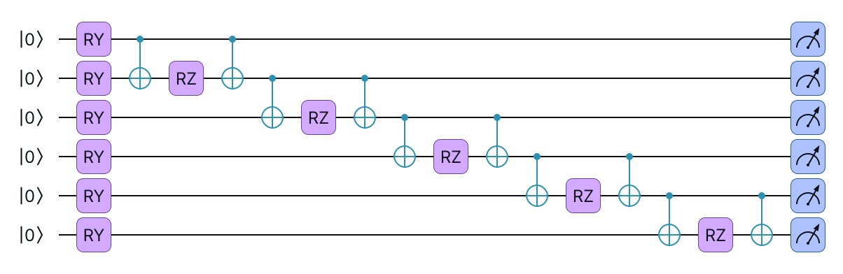
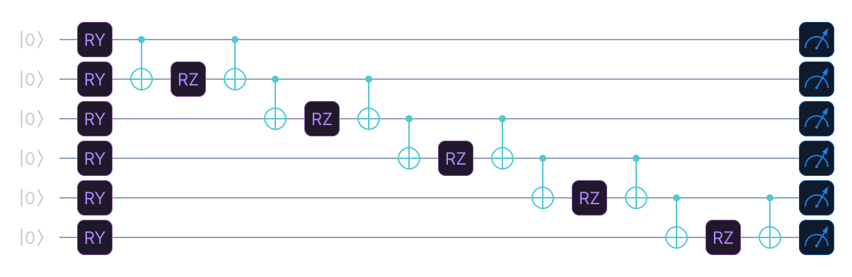
A hand-built ZZ-style feature map (light theme)

One such map: RY(x_q) embeds one feature per qubit, then a CNOT-RZ-CNOT block acts on each pair of neighbouring qubits, which is the usual way to write a two-qubit interaction into a feature map. It has six qubits, six features and one repetition.

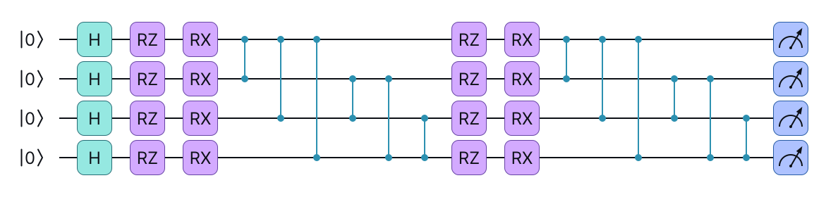
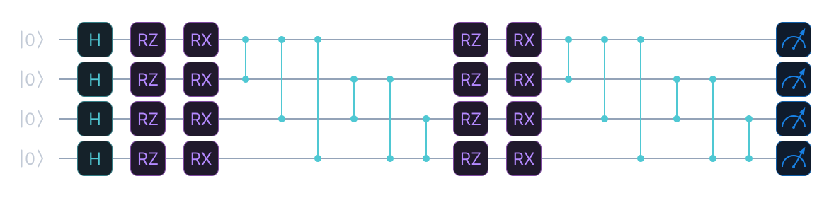
A hand-built instantaneous quantum polynomial feature map (light theme)

Another map, with two repetitions: a layer of Hadamard gates, RZ and RX rotations that carry the data, and CZ gates across every pair of qubits instead of along a ladder, then the rotations and the entangling gates once more. Neither of these two maps is "Angle" or "AngleCNOT". Both are the kind of map that you build with CircuitBuilder and pass to QuantumKernel(feature_map=...).

For custom observables based on fidelity (swap tests, the Bures distance and so on), call circuit.zero_state_probability(weights, inputs) directly. It returns the probability of the all-zeros state without going through the Pauli machinery:

from eigenkit import Circuit, CircuitBuilder
from eigenkit.core.ir import Negate

qc = CircuitBuilder(n_qubits=2)
x = qc.add_inputs(2)
for q in range(2):
    qc.rx(x[q], qubit=q)
for q in reversed(range(2)):
    qc.rx(Negate(x[q]), qubit=q)
spec = qc.build()

circuit = Circuit(blocks=spec)
# The inversion circuit has no trainable weights, so pass an empty weight vector.
print(circuit.zero_state_probability([], [0.4, -0.2]))  # ~1.0 (U U^dag)

API reference

`eigenkit.qml._kernels.QuantumKernel`

Quantum kernel matrix K[i, j] = fidelity(U(x_i), U(x_j)).

Parameters:

Name	Type	Description	Default
`n_features`	`int`	The number of features. For the built-in maps, it is also the number of qubits.	required
`feature_map`	`FeatureMapLike`	The feature map. It is `"Angle"`, `"AngleCNOT"`, or a custom forward map `U(x; w)`. A custom map is a `CircuitSpec`, a `CircuitBuilder`, a block, a list of blocks, or a callable `emit(builder, x, w)` that writes the map onto a `CircuitBuilder`, given the input references `x` and the weight references `w`. A custom map must read exactly `n_features` inputs. Default: `"AngleCNOT"`.	`'AngleCNOT'`
`reps`	`int`	The number of repetitions of a built-in feature map. `reps=1` uses only the `RX` encoding, and `reps>=2` adds repetitions of the `RZ` encoding (with ladders of controlled-NOT (CNOT) gates for `"AngleCNOT"`). It is ignored for a custom map. Default: `2`.	`2`
`provider`	`ProviderSpec`	The backend. It takes the same options as `Circuit(provider=...)`. Default: `"numpy"`, which needs no extra.	`'numpy'`
`weights`	`Sequence[float] \| ndarray \| None`	The trainable weights of the feature map, of shape `(n_weights,)`. `None` uses zeros. Maps without weights ignore them.	`None`
`scale`	`float`	The bandwidth. Every input is multiplied by it before it reaches the circuit, so `scale` sets how far apart two samples are in Hilbert space. Default: `1.0`.	`1.0`
`n_weights`	`int \| None`	The number of weights that a callable `feature_map` reserves. For any other map, it is read from the circuit and, if given, checked.	`None`
`n_qubits`	`int \| None`	The number of qubits of a callable `feature_map`. Default: `n_features`.	`None`
`psd_projection`	`bool`	If True, a sampled Gram matrix is projected onto the nearest positive semidefinite matrix. It only affects backends that use shots. Default: `False`.	`False`

Example

import numpy as np
from eigenkit import QuantumKernel

rng = np.random.default_rng(0)
X_train, X_test = rng.uniform(0, np.pi, (8, 4)), rng.uniform(0, np.pi, (3, 4))

qk = QuantumKernel(n_features=4, feature_map="AngleCNOT", reps=2)
K_train = qk.compute_kernel_matrix(X_train)
K_test = qk.compute_kernel_matrix(X_test, X_train)

# A custom feature map with a trainable weight.
def zz_map(qc, x, w):
    for q in range(len(x)):
        qc.ry(w[0], q)
        qc.h(q)
        qc.rz(x[q], q)
    qc.pauli_exponential([("Z", 0), ("Z", 1)], x[0])

trainable = QuantumKernel(n_features=2, feature_map=zz_map, n_weights=1)
K = trainable.compute_kernel_matrix(X_train[:, :2], weights=[0.3])

`circuit` `property`

The compiled inversion circuit.

A backend with shots runs it for each kernel entry. It is compiled when it is first accessed.

`feature_map_circuit` `property`

The compiled forward feature map U(x; w).

It is compiled when it is first accessed.

`feature_map_spec` `property`

The forward feature map U(x; w), as a CircuitSpec.

`kernel_spec` `property`

The inversion circuit U(x_1; w) U(x_2; w)^dagger, as a CircuitSpec.

It has 2 * n_features inputs.

`n_qubits` `property`

The number of qubits of the feature-map circuit.

`n_weights` `property`

The number of trainable weights in the feature map.

`__sklearn_clone__()`

Return a new copy of the kernel, not compiled yet, for sklearn.base.clone.

GridSearchCV, cross_val_score and Pipeline use it. The copy has the same feature map, provider, weights, scale and psd_projection.

`compute_kernel_matrix(X, Y=None, *, weights=None)`

Return the kernel matrix between the rows of X and the rows of Y.

Parameters:

Name	Type	Description	Default
`X`	`ndarray`	The samples, of shape `(n_X, n_features)`.	required
`Y`	`ndarray \| None`	The second set of samples, of shape `(n_Y, n_features)`. If `None`, the method returns `K(X, X)`.	`None`
`weights`	`ndarray \| None`	The feature-map weights for this evaluation. By default, they are the kernel's own `weights`, or zeros if it has none.	`None`

Returns:

Type	Description
`ndarray`	An array of shape `(n_X, n_Y)`.

`draw(*, inversion=False, decimals=3)`

Return a text drawing of the feature map, or of the inversion circuit.

Parameters:

Name	Type	Description	Default
`inversion`	`bool`	If True, draw `U(x_1) U(x_2)^dagger` instead of `U(x)`.	`False`
`decimals`	`int`	The number of significant digits of constant angles.	`3`

Returns:

Type	Description
`str`	The drawing, as a string of several lines.

`draw_mpl(*, inversion=False, **kwargs)`

Draw the feature map, or the inversion circuit, with Matplotlib.

The inversion circuit is drawn with a measurement on every qubit, and the forward map without one. This method needs the viz extra.

Parameters:

Name	Type	Description	Default
`inversion`	`bool`	If True, draw `U(x_1) U(x_2)^dagger` instead of `U(x)`.	`False`
`**kwargs`	`Any`	Arguments passed to `draw_mpl()`, for example `style="eigen"`.	`{}`

Returns:

Type	Description
`'tuple[Figure, Axes]'`	The Matplotlib figure and axes, as the pair `(fig, ax)`.

`estimate_cost(X, Y=None)`

Return what computing K(X, Y) would need on the backend of this kernel.

Nothing is submitted. On a sampling backend, the inversion circuit is compiled (and transpiled, for hardware) to report its size.

Parameters:

Name	Type	Description	Default
`X`	`ndarray`	The samples, of shape `(n_X, n_features)`.	required
`Y`	`ndarray \| None`	The second set of samples, of shape `(n_Y, n_features)`, or `None` for the Gram matrix `K(X, X)`.	`None`

Returns:

Type	Description
`dict`	A dictionary with the keys `method` (`"statevector"` or `"inversion"`), `n_circuits`, `n_jobs`, `shots` and `total_shots`. With the `"statevector"` method, it also has `n_state_evolutions`. When the backend reports them, it also has the transpiled two-qubit gate count `n_2q_gates`, the `depth` and the `backend_name`.

`from_json_dict(data, provider=None)` `classmethod`

Rebuild a kernel written by to_json_dict().

Parameters:

Name	Type	Description	Default
`data`	`dict`	The stored description.	required
`provider`	`ProviderSpec \| None`	A provider that replaces the stored one. It is needed when the stored provider held a secret, or to move a saved model onto another backend.	`None`

Returns:

Type	Description
`'QuantumKernel'`	The rebuilt kernel.

`kernel_value(x1, x2, *, weights=None)`

Return the kernel value of one pair (x1, x2), from the inversion circuit.

`retrieve_kernel_matrix(job, n_x=None, n_y=None)`

Reconnect to a kernel job submitted earlier, possibly in another session.

Parameters:

Name	Type	Description	Default
`job`	`str \| Path`	The JSON file written by `KernelJob.save()`, or a job id on its own.	required
`n_x`	`int \| None`	The number of rows of the matrix. It is required with a job id on its own.	`None`
`n_y`	`int \| None`	The number of columns, for a rectangular matrix. Leave it as `None` for a Gram matrix.	`None`

Returns:

Type	Description
`KernelJob`	A `KernelJob`. Call `.result()` on it to get the matrix.

`submit_kernel_matrix(X, Y=None, *, weights=None)`

Submit K(X, Y) as one asynchronous job, and return its handle.

This is for the queues of a quantum processing unit (QPU), which can take minutes or hours. Print the job id of the handle or call its save(), and collect the matrix later with job.result() or, from a new session, with retrieve_kernel_matrix().

Parameters:

Name	Type	Description	Default
`X`	`ndarray`	The samples, of shape `(n_X, n_features)`.	required
`Y`	`ndarray \| None`	The second set of samples, of shape `(n_Y, n_features)`, or `None` for the Gram matrix.	`None`
`weights`	`ndarray \| None`	The feature-map weights. By default, they are the kernel's own.	`None`

Returns:

Type	Description
`KernelJob`	A `KernelJob`.

Raises:

Type	Description
`NotImplementedError`	On backends without asynchronous submission, which includes every local simulator. Use `compute_kernel_matrix()` on them.

`to_json_dict()`

Return a JSON description of the kernel, for .eigenkit bundles.

A custom feature map is stored as its CircuitSpec. Secret fields of the provider, such as access tokens, are never written.

Returns:

Type	Description
`dict`	The description, as a dictionary.

`with_weights(weights)`

Return a copy of this kernel with different trainable weights.

Parameters:

Name	Type	Description	Default
`weights`	`ndarray`	The new weights, of shape `(n_weights,)`.	required

Returns:

Type	Description
`'QuantumKernel'`	A new kernel, which is not compiled yet.

`eigenkit.qml._kernels.KernelJob`

A kernel matrix submitted to a backend, to be collected later.

QuantumKernel.submit_kernel_matrix() returns it. The handle records which pair each submitted circuit measured, so result() returns the assembled matrix instead of a flat list of probabilities. save() writes this information together with the job id, so that the matrix can be collected from a new session with QuantumKernel.retrieve_kernel_matrix().

`n_circuits` `property`

The number of circuits that the job runs, one for each measured entry.

`job_id()`

Return the identifier of the job on the backend.

`result()`

Wait until the job finishes, and return the kernel matrix.

Returns:

Type	Description
`ndarray`	The kernel matrix, of shape `(n_x, n_x)` for a Gram matrix and `(n_x, n_y)` otherwise.

`save(path)`

Write the job id and the layout of the pairs to a JSON file.

The setting of psd_projection is written too.

Parameters:

Name	Type	Description	Default
`path`	`str \| Path`	Where to write the file. Its suffix is replaced by `.json`, or `.json` is added when it has none.	required

Returns:

Type	Description
`Path`	The path of the written file.

`status()`

Return the current status of the job, as a string from the backend.

`eigenkit.qml._alignment.align_kernel(kernel, X, y, *, loss='svc', optimizer='spsa', maxiter=50, C=1.0, initial_weights=None, learning_rate=None, perturbation=0.2, random_state=0, callback=None)`

Train the weights of a kernel so that it fits the labels.

Parameters:

Name	Type	Description	Default
`kernel`	`QuantumKernel`	A `QuantumKernel` whose feature map has trainable weights.	required
`X`	`ndarray`	The training samples, of shape `(n, n_features)`.	required
`y`	`ndarray`	The training labels, of shape `(n,)`.	required
`loss`	`str \| Callable[[ndarray, ndarray], float]`	The loss to minimise. It is `"svc"` (the dual objective of the support vector machine, which is the loss of quantum kernel alignment), `"kta"` (minus the kernel-target alignment), or a callable `loss(K, y) -> float`.	`'svc'`
`optimizer`	`str \| Callable`	The optimiser. It can be `"spsa"`, the default, which selects Simultaneous Perturbation Stochastic Approximation (SPSA). It can also be the name of a `scipy.optimize.minimize` method such as `"COBYLA"`, or a callable `optimizer(fun, x0) -> x`.	`'spsa'`
`maxiter`	`int`	The number of SPSA iterations, or the `maxiter` option of SciPy.	`50`
`C`	`float`	The regularisation parameter of the support vector machine, for the `"svc"` loss.	`1.0`
`initial_weights`	`ndarray \| None`	The starting point. By default, it is the kernel's own weights, or zeros if the kernel has none.	`None`
`learning_rate`	`float \| None`	The initial step size of SPSA. `None` calibrates it so that the first step moves the weights by about `2π / 10`. The `"svc"` loss grows with the number of samples, so a fixed step that suits one dataset size can be far too large for another.	`None`
`perturbation`	`float`	The initial perturbation size of SPSA. The default, `0.2`, is the value that qiskit-algorithms uses for its calibration. Much smaller values give estimates of the gradient that are too local to cross a flat region of the loss.	`0.2`
`random_state`	`int \| None`	The seed for the perturbation directions of SPSA.	`0`
`callback`	`Callable[[int, ndarray, float], None] \| None`	A function called as `callback(iteration, weights, loss)` after every SPSA iteration or SciPy evaluation.	`None`

Returns:

Type	Description
`KernelAlignmentResult`	A `KernelAlignmentResult`.

Raises:

Type	Description
`ValueError`	If the kernel has no trainable weights, or if `loss` is an unknown name.

Example

import numpy as np
from eigenkit import QSVC, QuantumKernel, align_kernel

def my_map(qc, x, w):
    for q in range(len(x)):
        qc.ry(w[0], q)
        qc.rz(x[q], q)

rng = np.random.default_rng(0)
X_train = rng.uniform(0, np.pi, (8, 2))
y_train = np.array([0, 1] * 4)

kernel = QuantumKernel(n_features=2, feature_map=my_map, n_weights=1)
result = align_kernel(kernel, X_train, y_train, maxiter=20)
model = QSVC(kernel=result.kernel).fit(X_train, y_train)

`eigenkit.qml._alignment.KernelAlignmentResult` `dataclass`

Outcome of align_kernel().

Attributes:

Name	Type	Description
`weights`	`ndarray`	The trained weights.
`kernel`	`QuantumKernel`	A copy of the input kernel with `weights`, ready for `QSVC(kernel=...)`.
`loss`	`float`	The loss at `weights`.
`initial_loss`	`float`	The loss at the starting weights.
`loss_history`	`tuple[float, ...]`	The loss after every iteration of Simultaneous Perturbation Stochastic Approximation (SPSA), or at every evaluation for a SciPy optimiser. With SPSA, `weights` is the point with the lowest loss seen, including the starting weights.
`n_evaluations`	`int`	The number of kernel matrices computed.
`success`	`bool`	Whether the loss is lower than at the starting point.

`eigenkit.qml._alignment.kernel_target_alignment(K, y)`

Return the kernel-target alignment <K, Y>_F / (||K||_F ||Y||_F).

Y_ij = +1 when y_i == y_j and -1 otherwise. For binary labels in {-1, +1}, this is y y^T.

Parameters:

Name	Type	Description	Default
`K`	`ndarray`	The Gram matrix, of shape `(n, n)`.	required
`y`	`ndarray`	The labels, of shape `(n,)`.	required

Returns:

Type	Description
`float`	A value in `[-1, 1]`. A higher value means that the kernel already separates the classes.

`eigenkit.qml._alignment.svc_dual_loss(K, y, C=1.0)`

Return the optimal dual objective of a support vector machine (SVM).

The SVM is fitted on a precomputed kernel. This is the "svc" loss.

Parameters:

Name	Type	Description	Default
`K`	`ndarray`	The training Gram matrix, of shape `(n, n)`.	required
`y`	`ndarray`	The labels, of shape `(n,)`. They must have exactly two classes.	required
`C`	`float`	The regularisation parameter of the SVM.	`1.0`

Returns:

Type	Description
`float`	The value `sum \|alpha_i y_i\| - 1/2 (alpha y)^T K_sv (alpha y)`, summed over the support vectors. Lower is better.

Raises:

Type	Description
`ValueError`	If `y` does not have exactly two classes. Use `loss="kta"` for more classes.

`eigenkit.qml._kernels.project_psd(K)`

Return the nearest positive semidefinite matrix to a symmetric K.

Shot noise can make a measured Gram matrix slightly indefinite, and a support vector machine solver handles such a matrix poorly. Setting the negative eigenvalues to zero gives the nearest positive semidefinite matrix in the Frobenius norm.

Parameters:

Name	Type	Description	Default
`K`	`ndarray`	A square, symmetric kernel matrix.	required

Returns:

Type	Description
`ndarray`	The projected matrix, of the same shape.

Quantum Kernels

Feature maps

Custom feature maps

Trainable kernels and kernel alignment

Bandwidth

How the kernel value is computed

On hardware

Choosing a backend

Use with scikit-learn estimators

Direct use of zero_state_probability

API reference

eigenkit.qml._kernels.QuantumKernel

circuit property

feature_map_circuit property

feature_map_spec property

kernel_spec property

n_qubits property

n_weights property

__sklearn_clone__()

compute_kernel_matrix(X, Y=None, *, weights=None)

draw(*, inversion=False, decimals=3)

draw_mpl(*, inversion=False, **kwargs)

estimate_cost(X, Y=None)

from_json_dict(data, provider=None) classmethod

kernel_value(x1, x2, *, weights=None)

retrieve_kernel_matrix(job, n_x=None, n_y=None)

submit_kernel_matrix(X, Y=None, *, weights=None)

to_json_dict()

with_weights(weights)

eigenkit.qml._kernels.KernelJob

n_circuits property

job_id()

result()

save(path)

status()

eigenkit.qml._alignment.align_kernel(kernel, X, y, *, loss='svc', optimizer='spsa', maxiter=50, C=1.0, initial_weights=None, learning_rate=None, perturbation=0.2, random_state=0, callback=None)

eigenkit.qml._alignment.KernelAlignmentResult dataclass

eigenkit.qml._alignment.kernel_target_alignment(K, y)

eigenkit.qml._alignment.svc_dual_loss(K, y, C=1.0)

eigenkit.qml._kernels.project_psd(K)

Direct use of `zero_state_probability`

`eigenkit.qml._kernels.QuantumKernel`

`circuit` `property`

`feature_map_circuit` `property`

`feature_map_spec` `property`

`kernel_spec` `property`

`n_qubits` `property`

`n_weights` `property`

`__sklearn_clone__()`

`compute_kernel_matrix(X, Y=None, *, weights=None)`

`draw(*, inversion=False, decimals=3)`

`draw_mpl(*, inversion=False, **kwargs)`

`estimate_cost(X, Y=None)`

`from_json_dict(data, provider=None)` `classmethod`

`kernel_value(x1, x2, *, weights=None)`

`retrieve_kernel_matrix(job, n_x=None, n_y=None)`

`submit_kernel_matrix(X, Y=None, *, weights=None)`

`to_json_dict()`

`with_weights(weights)`

`eigenkit.qml._kernels.KernelJob`

`n_circuits` `property`

`job_id()`

`result()`

`save(path)`

`status()`

`eigenkit.qml._alignment.align_kernel(kernel, X, y, *, loss='svc', optimizer='spsa', maxiter=50, C=1.0, initial_weights=None, learning_rate=None, perturbation=0.2, random_state=0, callback=None)`

`eigenkit.qml._alignment.KernelAlignmentResult` `dataclass`

`eigenkit.qml._alignment.kernel_target_alignment(K, y)`

`eigenkit.qml._alignment.svc_dual_loss(K, y, C=1.0)`

`eigenkit.qml._kernels.project_psd(K)`