Usage example: Generic Estimators

GenericClassifier and GenericRegressor are wrappers, compatible with sklearn, that train any torch.nn.Module through the standard fit and predict interface of the library. HQNC and HQNR build the architecture of the model for you. The generic estimators instead expect a complete network, output head included, so you have full control over the architecture.

This example has two parts:

Classification: the moons dataset, which has two classes, with a hybrid model that is part quantum and part classical.
Regression: the diabetes dataset, with a hybrid model that uses a quantum layer to extract features.

Imports

import matplotlib
import matplotlib.pyplot as plt
import numpy as np
from sklearn.model_selection import train_test_split
import torch
from torch import nn

from eigenkit import GenericClassifier, GenericRegressor
from eigenkit.datasets import STYLE_COLORS, load_dataset, rc_params
from eigenkit import Basic, Reupload

Part 1: Classification

Data

The moons dataset is a small benchmark with two features and two classes. Its decision boundary is small and non-linear, which makes it a good fit for hybrid models.

data = load_dataset("moons")
X_train, y_train = data["X_train"], data["y_train"]
X_test, y_test = data["X_test"], data["y_test"]

X_fit, X_val, y_fit, y_val = train_test_split(
    X_train,
    y_train,
    test_size=0.2,
    stratify=y_train,
    random_state=42,
)

print(f"Train: {X_fit.shape}, Validation: {X_val.shape}, Test: {X_test.shape}")
print(f"Classes: {np.unique(y_train)}")

Train: (128, 2), Validation: (32, 2), Test: (40, 2)
Classes: [0 1]

Build a hybrid model

The model is a small nn.Sequential. A linear layer expands the two input features to the number of qubits, Basic processes these values, and the last linear layer maps the result to two logits, one for each class.

Basic takes n_qubits inputs and returns n_qubits outputs, so the sizes of the layers on both sides must match.

N_QUBITS = 5
N_CLASSES = 2

torch.manual_seed(42)
quantum_layer = Basic(n_qubits=N_QUBITS, depth=3, variational_type="strong")

clf_net = nn.Sequential(
    nn.Linear(2, N_QUBITS),  # expand features to qubit count
    nn.ReLU(),
    quantum_layer,  # (batch, N_QUBITS) -> (batch, N_QUBITS) expectation values
    nn.Linear(N_QUBITS, N_CLASSES),
)

print(clf_net)

Sequential(
  (0): Linear(in_features=2, out_features=5, bias=True)
  (1): ReLU()
  (2): Basic(
    (circuit): TorchCircuit()
  )
  (3): Linear(in_features=5, out_features=2, bias=True)
)

Train with `GenericClassifier`

GenericClassifier wraps the network in a standard sklearn estimator. Pass the complete nn.Module as model. Set in_features, so that the wrapper checks the shape of the input in fit(). Configure the training loop with epochs, lr and batch_size.

The wrapper encodes the labels automatically, so y_train can hold integers, strings or any other hashable labels.

Pre-trained weights and the behaviour of fit()

fit() does not start from the weights that the nn.Module holds. It copies the module, and then calls reset_parameters() on every submodule that has this method (such as nn.Linear and the quantum layers of eigenkit), seeded with random_state. So the weights of these layers are drawn again before training, even if the module that you pass already holds trained weights. The module that you pass is not changed. clone() copies the hyperparameters of the estimator, not the trained weights, and each later call to fit() (for example after clone(), or inside cross-validation) also starts again from new weights. To keep the trained weights, use the fitted estimator, or save it with save() and load it again with load(), and do not call fit() on it again.

clf = GenericClassifier(
    model=clf_net,
    in_features=2,
    epochs=150,
    lr=0.01,
    batch_size=16,
    random_state=42,
)

clf.fit(X_fit, y_fit, X_val=X_val, y_val=y_val)
print(f"Test accuracy: {clf.score(X_test, y_test):.3f}")

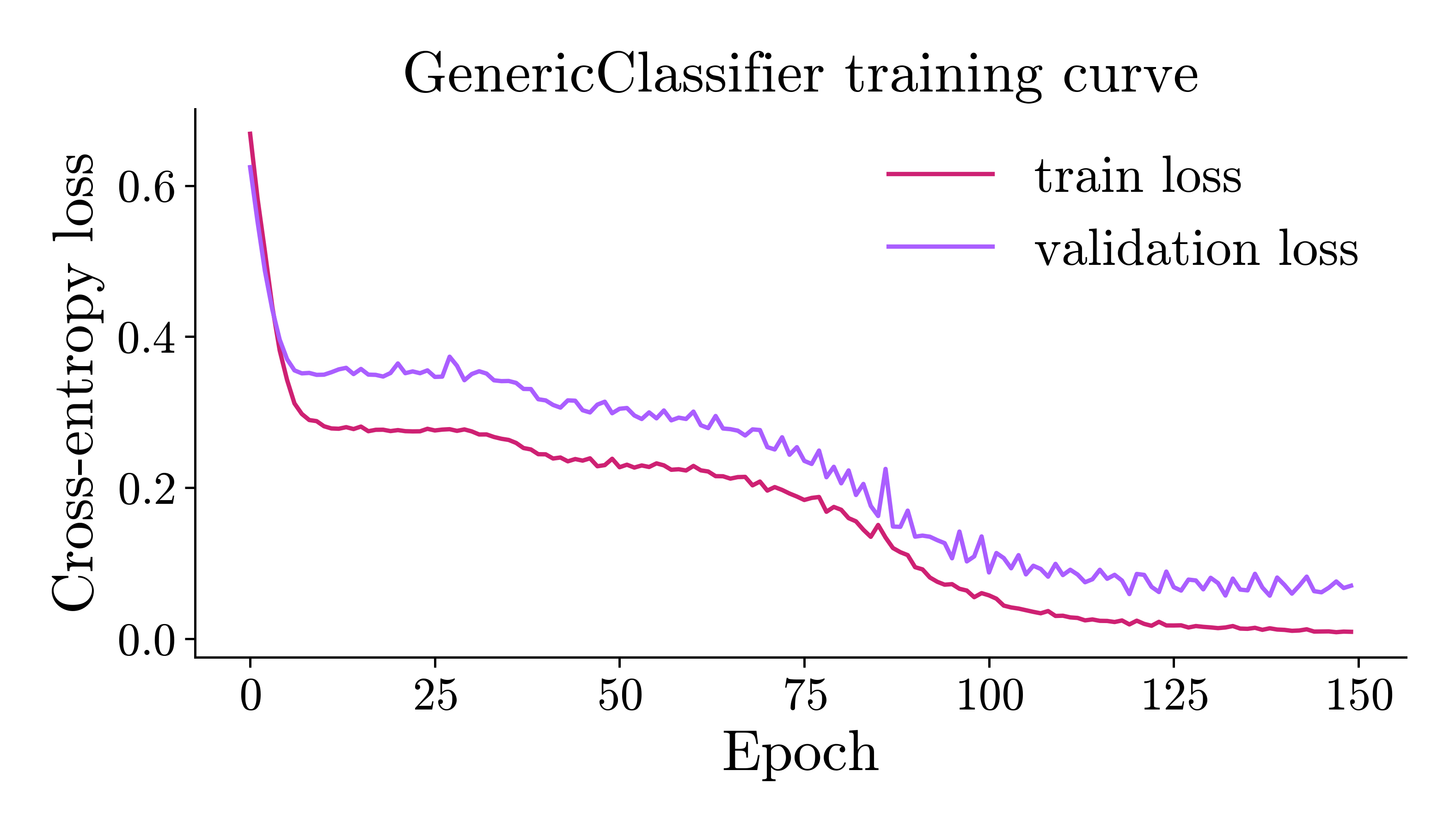
GenericClassifier training | Epoch 1/150 | loss=0.668630 | val_loss=0.624434 | elapsed=0.2s | eta=32.6s
GenericClassifier training | Epoch 2/150 | loss=0.583259 | val_loss=0.552643 | elapsed=0.4s | eta=33.1s
GenericClassifier training | Epoch 3/150 | loss=0.512898 | val_loss=0.487117 | elapsed=0.7s | eta=34.2s
...
GenericClassifier training | Epoch 149/150 | loss=0.009535 | val_loss=0.067237 | elapsed=56.7s | eta=0.4s
GenericClassifier training | Epoch 150/150 | loss=0.009276 | val_loss=0.070270 | elapsed=56.9s | eta=0.0s
Test accuracy: 1.000

Training curve

for theme in ("light", "dark"):
    with matplotlib.rc_context(rc_params(theme=theme)):
        fig, ax = plt.subplots(figsize=(7, 4))
        ax.plot(clf.train_losses_, color=STYLE_COLORS[0], label="train loss")
        ax.plot(clf.validation_losses_, color=STYLE_COLORS[1], label="validation loss")
        ax.set_xlabel("Epoch")
        ax.set_ylabel("Cross-entropy loss")
        ax.set_title("GenericClassifier training curve")
        ax.legend()
        fig.tight_layout()
        fig.savefig(f"generic_classifier_training_curve_{theme}.png")
        if theme == "light":
            plt.show()
        else:
            plt.close(fig)

png png

Predict and inspect outputs

labels = clf.predict(X_test)
probs = clf.predict_proba(X_test)

print("Predicted labels (first 8):", labels[:8].tolist())
print("Class probabilities (first 3):")
print(probs[:3])

Predicted labels (first 8): [0, 1, 1, 1, 0, 1, 0, 1]
Class probabilities (first 3):
[[9.9979252e-01 2.0752900e-04]
 [1.8817510e-02 9.8118252e-01]
 [3.3264074e-01 6.6735923e-01]]

Save and load

Call save() after training. The bundle stores the trained weights, the label encoder and the training metadata.

The architecture cannot be rebuilt automatically from the bundle, so you must pass a module with the same nn.Module structure to GenericClassifier.load(). The saved weights are loaded into a copy of this module, and the module that you pass is not changed. So the module used in training and the module passed to load() do not need to be the same Python object. They only need to have the same structure of layers.

clf.save("clf_hybrid.eigenkit")

# Rebuild the architecture (same structure, fresh weights)
clf_net_fresh = nn.Sequential(
    nn.Linear(2, N_QUBITS),
    nn.ReLU(),
    Basic(n_qubits=N_QUBITS, depth=3, variational_type="strong"),
    nn.Linear(N_QUBITS, N_CLASSES),
)

clf_loaded = GenericClassifier.load("clf_hybrid.eigenkit", model=clf_net_fresh)

# Predictions must match the original model
assert (clf_loaded.predict(X_test) == clf.predict(X_test)).all()
print(f"Loaded model test accuracy: {clf_loaded.score(X_test, y_test):.3f}")

Loaded model test accuracy: 1.000

Part 2: Regression

Data

The diabetes dataset has 10 features, and its target is a continuous measure of the progression of the disease. We normalise both the features and the target with StandardScaler.

from sklearn.preprocessing import StandardScaler

data = load_dataset("diabetes")
X_train_r_full, y_train_r_full = data["X_train"], data["y_train"]
X_test_r, y_test_r_raw = data["X_test"], data["y_test"]

X_train_r_raw, X_val_r_raw, y_train_r_raw, y_val_r_raw = train_test_split(
    X_train_r_full,
    y_train_r_full,
    test_size=0.2,
    random_state=42,
)

x_scaler = StandardScaler()
X_train_r = x_scaler.fit_transform(X_train_r_raw).astype(np.float32)
X_val_r = x_scaler.transform(X_val_r_raw).astype(np.float32)
X_test_r = x_scaler.transform(X_test_r).astype(np.float32)

y_scaler = StandardScaler()
y_train_r = (
    y_scaler.fit_transform(y_train_r_raw.reshape(-1, 1)).ravel().astype(np.float32)
)
y_val_r = y_scaler.transform(y_val_r_raw.reshape(-1, 1)).ravel().astype(np.float32)
y_test_r = y_scaler.transform(y_test_r_raw.reshape(-1, 1)).ravel().astype(np.float32)

print(f"Train: {X_train_r.shape}, Validation: {X_val_r.shape}, Test: {X_test_r.shape}")
print(f"Target mean: {y_train_r.mean():.3f}, std: {y_train_r.std():.3f}")

Train: (282, 10), Validation: (71, 10), Test: (89, 10)
Target mean: -0.000, std: 1.000

Build a hybrid regression model

The architecture has three parts:

A classical encoder, which compresses the 10 features to the number of qubits.
A Basic quantum layer, which is a variational layer that extracts features.
A classical regression head, which is a linear output with a single neuron.

GenericRegressor expects the forward() method of the model to return a tensor of shape (batch,) or (batch, 1). The last layer, nn.Linear(N_QUBITS_R, 1), meets this requirement.

N_QUBITS_R = 6
IN_FEATURES_R = X_train_r.shape[1]  # 10

torch.manual_seed(42)
quantum_layer_r = Basic(n_qubits=N_QUBITS_R, depth=3, variational_type="strong")

reg_net = nn.Sequential(
    nn.Linear(IN_FEATURES_R, N_QUBITS_R),
    nn.ReLU(),
    quantum_layer_r,
    nn.Linear(N_QUBITS_R, 1),
)

print(reg_net)

Sequential(
  (0): Linear(in_features=10, out_features=6, bias=True)
  (1): ReLU()
  (2): Basic(
    (circuit): TorchCircuit()
  )
  (3): Linear(in_features=6, out_features=1, bias=True)
)

Train with `GenericRegressor`

The default loss is the mean squared error (MSE). Pass loss_func="mae" (the mean absolute error) or loss_func="huber" (the Huber loss) to use another loss, or pass any callable (output, target) -> scalar_tensor for a custom loss.

reg = GenericRegressor(
    model=reg_net,
    in_features=IN_FEATURES_R,
    loss_func="mse",
    epochs=100,
    lr=0.001,
    batch_size=32,
    random_state=42,
)

reg.fit(X_train_r, y_train_r, X_val=X_val_r, y_val=y_val_r)
print(f"Test R²: {reg.score(X_test_r, y_test_r):.3f}")

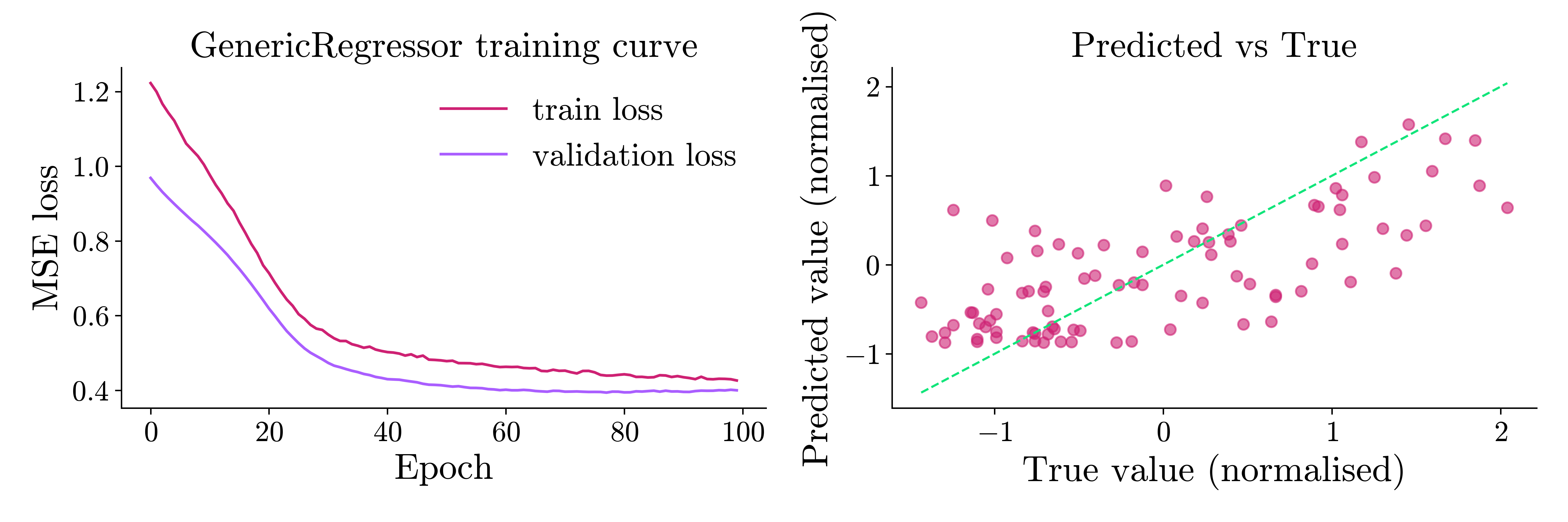
GenericRegressor training | Epoch 1/100 | loss=1.222554 | val_loss=0.968641 | elapsed=0.2s | eta=23.3s
GenericRegressor training | Epoch 2/100 | loss=1.199555 | val_loss=0.949176 | elapsed=0.5s | eta=22.2s
GenericRegressor training | Epoch 3/100 | loss=1.166938 | val_loss=0.930964 | elapsed=0.7s | eta=21.9s
...
GenericRegressor training | Epoch 99/100 | loss=0.429658 | val_loss=0.401382 | elapsed=27.2s | eta=0.3s
GenericRegressor training | Epoch 100/100 | loss=0.426311 | val_loss=0.400020 | elapsed=27.4s | eta=0.0s
Test R²: 0.489

Training curve and predictions

preds = reg.predict(X_test_r)

for theme in ("light", "dark"):
    with matplotlib.rc_context(rc_params(theme=theme)):
        fig, axes = plt.subplots(1, 2, figsize=(12, 4))

        axes[0].plot(reg.train_losses_, color=STYLE_COLORS[0], label="train loss")
        axes[0].plot(
            reg.validation_losses_, color=STYLE_COLORS[1], label="validation loss"
        )
        axes[0].set_xlabel("Epoch")
        axes[0].set_ylabel("MSE loss")
        axes[0].set_title("GenericRegressor training curve")
        axes[0].legend()

        lims = [min(y_test_r.min(), preds.min()), max(y_test_r.max(), preds.max())]
        axes[1].scatter(y_test_r, preds, alpha=0.6, color=STYLE_COLORS[0])
        axes[1].plot(lims, lims, "--", linewidth=1.2, color=STYLE_COLORS[5])
        axes[1].set_xlabel("True value (normalised)")
        axes[1].set_ylabel("Predicted value (normalised)")
        axes[1].set_title("Predicted vs True")

        plt.tight_layout()
        fig.savefig(f"generic_regressor_training_curve_{theme}.png")
        if theme == "light":
            plt.show()
        else:
            plt.close(fig)

png png

Save and load

Saving and loading work as for the classifier. Call save() after training, and pass the architecture again when you load. The bundle stores the weights and the training metadata, but not the architecture.

reg.save("reg_hybrid.eigenkit")

# Rebuild the architecture (same structure, fresh weights)
reg_net_fresh = nn.Sequential(
    nn.Linear(IN_FEATURES_R, N_QUBITS_R),
    nn.ReLU(),
    Basic(n_qubits=N_QUBITS_R, depth=3, variational_type="strong"),
    nn.Linear(N_QUBITS_R, 1),
)

reg_loaded = GenericRegressor.load("reg_hybrid.eigenkit", model=reg_net_fresh)

np.testing.assert_allclose(
    reg_loaded.predict(X_test_r),
    reg.predict(X_test_r),
    atol=1e-5,
)
print(f"Loaded model R²: {reg_loaded.score(X_test_r, y_test_r):.3f}")

Loaded model R²: 0.489

Custom loss function

Any callable (output, target) -> scalar_tensor can be used directly as the loss. Note that a model trained with a callable loss cannot be saved: save() raises a SerializationError. Use a loss given by its name ("mse", "mae" or "huber") when you need to save the model.

The log-cosh loss is a smooth approximation of the MAE, and it is less sensitive to outliers than the MSE. The direct formula torch.log(torch.cosh(x)) overflows for |x| > 88 in float32, so we use the identity log(cosh(x)) = |x| + log(1 + exp(-2|x|)) - log(2), which stays finite for any input.

def log_cosh_loss(output, target):
    """Numerically stable log-cosh loss.

    Uses the identity log(cosh(x)) = |x| + log(1 + exp(-2|x|)) - log(2).
    """
    diff = output.squeeze(-1) - target
    abs_diff = torch.abs(diff)
    return (
        abs_diff + torch.log1p(torch.exp(-2.0 * abs_diff)) - torch.log(torch.tensor(2.0))
    ).mean()


torch.manual_seed(42)
reg_custom = GenericRegressor(
    model=nn.Sequential(
        nn.Linear(IN_FEATURES_R, N_QUBITS_R),
        nn.ReLU(),
        Basic(n_qubits=N_QUBITS_R, depth=3, variational_type="strong"),
        nn.Linear(N_QUBITS_R, 1),
    ),
    in_features=IN_FEATURES_R,
    loss_func=log_cosh_loss,
    epochs=30,
    lr=0.01,
)

reg_custom.fit(X_train_r, y_train_r, X_val=X_val_r, y_val=y_val_r)
print(f"Log-cosh model R²: {reg_custom.score(X_test_r, y_test_r):.3f}")

GenericRegressor training | Epoch 1/30 | loss=0.407534 | val_loss=0.307214 | elapsed=0.2s | eta=7.2s
GenericRegressor training | Epoch 2/30 | loss=0.317115 | val_loss=0.247753 | elapsed=0.5s | eta=6.6s
GenericRegressor training | Epoch 3/30 | loss=0.252423 | val_loss=0.213302 | elapsed=0.7s | eta=6.3s
...
GenericRegressor training | Epoch 29/30 | loss=0.158274 | val_loss=0.195311 | elapsed=6.0s | eta=0.2s
GenericRegressor training | Epoch 30/30 | loss=0.157571 | val_loss=0.191838 | elapsed=6.2s | eta=0.0s
Log-cosh model R²: 0.492

Usage example: Generic Estimators

Imports

Part 1: Classification

Data

Build a hybrid model

Train with GenericClassifier

Training curve

Predict and inspect outputs

Save and load

Part 2: Regression

Data

Build a hybrid regression model

Train with GenericRegressor

Training curve and predictions

Save and load

Custom loss function

Train with `GenericClassifier`

Train with `GenericRegressor`