Quantum Chemistry

eigenkit.chemistry computes ground-state energies. The process always has the same four steps: build a fermionic Hamiltonian, map it onto qubits, choose an ansatz, and minimise the energy with the Variational Quantum Eigensolver (VQE). Each step is a separate function, so you can stop after any of them and inspect the result.

Like optimization and reservoir, this package belongs to the core of the library. It uses only NumPy and SciPy, and needs neither PyTorch nor a backend package, so most of it runs on a bare installation. The exceptions are the functions that call external chemistry software: molecular_hamiltonian, hydrogen_molecule and bravyi_kitaev. They need the chemistry extra (pip install eigenkit[chemistry]), which installs PySCF, OpenFermion and openfermionpyscf.

The whole process in one example

The two-site Fermi-Hubbard model, also called the Fermi-Hubbard dimer, is the smallest model worth solving, and it needs no external software. This example solves it from start to finish and compares the result with the exact answer:

from eigenkit.chemistry import (
    VQE,
    exact_ground_state_energy,
    fermi_hubbard_dimer,
    jordan_wigner,
)

hamiltonian = fermi_hubbard_dimer(t=1.0, u=2.0)  # 6 fermionic terms
observable, offset = jordan_wigner(hamiltonian)  # 10 Pauli terms, offset 1.0

result = VQE(layers=3, restarts=5).solve(observable, 4, offset=offset)
exact = exact_ground_state_energy(observable, 4, offset=offset)

print(result.energy)  # -1.236068
print(exact)  # -1.236068
print(result.success)  # True

The model uses 4 qubits, two spin-orbitals per site. VQE uses provider="numpy" by default, so this example runs with no optional dependencies.

The rest of this page goes through the four steps one at a time.

Building a Hamiltonian

A FermionOperator is a dictionary of fermionic terms and their coefficients. Each term is a tuple of (mode, kind) pairs, where kind is 1 for a creation operator and 0 for an annihilation operator. For example, ((0, 1), (2, 0)) is c†₀c₂:

from eigenkit.chemistry import FermionOperator, fermi_hubbard_dimer

hamiltonian = fermi_hubbard_dimer(t=1.0, u=2.0)

for term, coeff in hamiltonian.terms.items():
    print(term, coeff)
# ((0, 1), (2, 0))                  (-1+0j)   hopping between the two sites
# ((2, 1), (0, 0))                  (-1+0j)
# ((1, 1), (3, 0))                  (-1+0j)
# ((3, 1), (1, 0))                  (-1+0j)
# ((0, 1), (0, 0), (1, 1), (1, 0))   (2+0j)   on-site repulsion, u
# ((2, 1), (2, 0), (3, 1), (3, 0))   (2+0j)

# The same notation builds one by hand: c†₀c₁ + c†₁c₀
hopping = FermionOperator({((0, 1), (1, 0)): 1.0, ((1, 1), (0, 0)): 1.0})
print(len(hopping.terms))  # 2

fermi_hubbard_dimer(t, u) uses only NumPy. t is the hopping amplitude between the two sites, and u is the on-site repulsion. Because it needs nothing else, it is the right model to develop against.

For real molecules, molecular_hamiltonian(geometry, basis=...) runs PySCF and OpenFermion, and hydrogen_molecule(bond_length) is a shortcut for H₂. Both return a Molecule. A Molecule holds the fermionic operator, the number of electrons and the nuclear repulsion energy, which are the values needed to turn a converged VQE energy into a physical one:

# Requires the `chemistry` extra: PySCF and OpenFermion.
from eigenkit.chemistry import hydrogen_molecule

molecule = hydrogen_molecule(bond_length=0.7414)
print(molecule.n_qubits, molecule.n_electrons)

Mapping onto qubits

A fermionic operator cannot be measured directly, so it has to be rewritten with Pauli operators. Both mappings return the same pair: an Observable and a scalar offset:

from eigenkit.chemistry import exact_ground_state_energy, jordan_wigner

observable, offset = jordan_wigner(hamiltonian)

print(len(observable.terms))  # 10
print(offset)  # 1.0
print(observable.terms[0])  # PauliTerm(coeff=-0.5, paulis=(('Y', 0), ('Z', 1), ('Y', 2)))

The offset must always be passed. It is the identity part of the Hamiltonian. It contains no Pauli operator, so it is left out of the observable. Pass it back in every time, otherwise every energy is wrong by a constant:

print(exact_ground_state_energy(observable, 4, offset=offset))  # -1.236068
print(exact_ground_state_energy(observable, 4))  # -2.236068

The two results differ by exactly 1.0, and nothing in the wrong one looks suspicious.

The two mappings have different dependencies, which is useful to know before you choose one. jordan_wigner is implemented in eigenkit and needs nothing else. bravyi_kitaev uses OpenFermion, and it raises ModuleNotFoundError without the chemistry extra. Jordan-Wigner is the natural default. Bravyi-Kitaev gives shorter Pauli strings for larger systems, at the cost of that dependency:

# Requires the `chemistry` extra: OpenFermion.
from eigenkit.chemistry import bravyi_kitaev

observable_bk, offset_bk = bravyi_kitaev(hamiltonian, n_qubits=4)
print(len(observable_bk.terms), offset_bk)

If you already work with OpenFermion, three functions convert between the two libraries. fermion_operator_from_openfermion and to_openfermion_fermion_operator convert fermionic operators in either direction, and observable_from_openfermion turns an openfermion.QubitOperator into the same (Observable, offset) pair that the mappings return. All three need OpenFermion.

Choosing an ansatz

The table compares the two ansätze that VQE supports: the hardware-efficient ansatz, and the unitary coupled-cluster ansatz with single and double excitations (UCCSD).

	Hardware-efficient	UCCSD
When it is used	By default	When you pass it with `ansatz=`
How it is built	A layer of `RY` rotations, then `layers` repetitions of a chain of `CNOT` gates and a pair of rotations	Single and double excitations, with a Trotter approximation, on a Hartree-Fock reference
Why you would choose it	A device can run it	The chemistry of the problem suggests it
Weights on `4` qubits with `2` electrons	`20` with `layers=2`	`10` with `reps=2`
Depth	Shallow	Much deeper for the same number of parameters
Reference state	None: it starts from `\|0…0⟩`	It adds `hartree_fock_state` at the start itself

By default, VQE builds a hardware-efficient ansatz: a layer of RY rotations, then layers repetitions of a chain of CNOT gates and a pair of rotations. hardware_efficient_ansatz builds the same circuit on its own, and hartree_fock_state builds the Hartree-Fock reference state that UCCSD starts from. Both are useful to count the parameters before you start a run:

from eigenkit.chemistry import hardware_efficient_ansatz, hartree_fock_state

print(hardware_efficient_ansatz(n_qubits=4, layers=2).n_weights)  # 20
print(hartree_fock_state(n_qubits=4, n_electrons=2).n_weights)  # 0, it is a fixed state

The ansatz designed for chemistry is uccsd_ansatz: a unitary coupled-cluster ansatz, with a Trotter approximation, built on the Hartree-Fock reference. Pass it explicitly:

from eigenkit.chemistry import uccsd_ansatz

ansatz = uccsd_ansatz(n_qubits=4, n_electrons=2, reps=2)
result = VQE(restarts=3).solve(observable, 4, offset=offset, ansatz=ansatz)

print(ansatz.n_weights)  # 10
print(result.energy)  # -1.236068

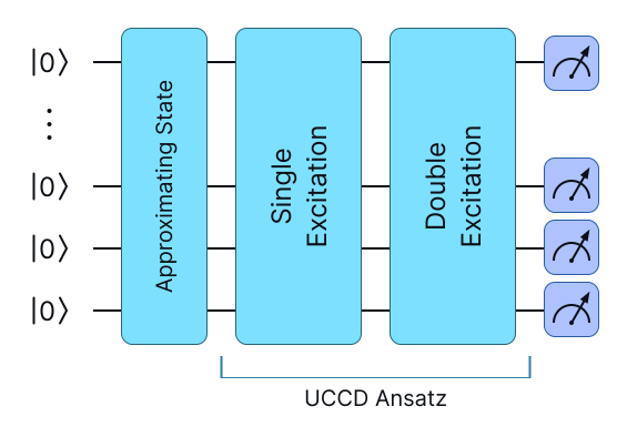
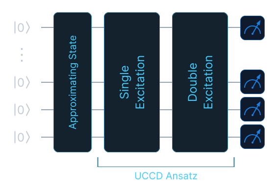
The UCCSD ansatz VQE optimises (light theme)

This figure draws the UCCSD column of the table above. The Hartree-Fock reference state is on the left. Then come the single and double excitations that uccsd_ansatz produces, with a Trotter approximation, and then the Pauli measurements whose weighted sum is the energy that VQE minimises. reps is the number of times the block of excitations is repeated. With one Trotter step, the ansatz converges to the first excited level, and with two it reaches the ground state.

The value of reps has a large effect. With reps=1, the ansatz has 5 parameters and converges to -1.0. This is not a near miss: it is the first excited level of this Hamiltonian, 0.236 above the ground state, and the result reports success=True. The optimiser did converge, but one Trotter step cannot reach the ground state. reps=2 doubles the number of parameters and reaches the exact energy.

For finer control, apply_hartree_fock(circuit, n_electrons) prepares the reference state on a CircuitBuilder that you are already building, and uccsd_excitation_generators(n_qubits, n_electrons) returns the generators T - T† themselves (5 of them for this system) if you want to build the ansatz in a different way.

Checking the answer

VQE gives an upper bound on the ground-state energy. For a system this small, you can compute the true value and see how close the bound is. dense_hamiltonian builds the matrix of the Hamiltonian, so the whole spectrum is available, and not only the lowest level:

import numpy as np
from eigenkit.chemistry import (
    dense_hamiltonian,
    fermi_hubbard_dimer_ground_energy,
)

matrix = dense_hamiltonian(observable, 4, offset=offset)

print(matrix.shape)  # (16, 16)
print(np.linalg.eigvalsh(matrix)[:3])  # [-1.236068 -1.  -1.]
print(fermi_hubbard_dimer_ground_energy(t=1.0, u=2.0))  # -1.236068

The second eigenvalue is where the UCCSD run with reps=1 above stopped. exact_ground_state_energy is the shortcut when only the lowest level is needed. For this model, the analytic formula at half filling agrees with the diagonalisation to the last digit, so three different methods give the same number.

Add this check to any workflow, because success=True only means that the optimiser converged; it does not mean that the energy is correct. Dense diagonalisation becomes impractical at around 14 qubits, where the matrix already needs about 4 gigabytes of memory. By then, you will have calibrated the ansatz on smaller cases where the check was possible.

API reference

`eigenkit.chemistry`

Quantum chemistry with the core of the library.

Build a fermionic Hamiltonian (FermionOperator), map it to a qubit Observable (jordan_wigner), and find its ground-state energy with the Variational Quantum Eigensolver (VQE), which uses the variational optimisation tools of the core. The package uses only NumPy and SciPy, needs no PyTorch, and works with any backend. For small systems, exact_ground_state_energy gives the classical reference value.

Example

from eigenkit.chemistry import (
    fermi_hubbard_dimer, jordan_wigner, VQE, exact_ground_state_energy,
)

hamiltonian, offset = jordan_wigner(fermi_hubbard_dimer(t=1.0, u=2.0))
result = VQE(layers=3, restarts=5).solve(hamiltonian, n_qubits=4, offset=offset)
exact = exact_ground_state_energy(hamiltonian, n_qubits=4, offset=offset)
print(result.energy, exact)

`FermionOperator`

A complex linear combination of fermionic terms, stored as {term: coeff}.

`init(terms=None)`

Build an operator from a mapping of terms to coefficients.

Parameters:

Name	Type	Description	Default
`terms`	`dict[Term, complex] \| None`	Maps each term to its coefficient. A term is a tuple of `(mode, action)` pairs, where `action` is `1` for creation and `0` for annihilation, applied from left to right. The empty tuple is the identity. The coefficients of repeated terms are added together. Leave it out for the zero operator. The default is `None`.	`None`

`annihilation(mode)` `classmethod`

The annihilation operator a_mode.

Parameters:

Name	Type	Description	Default
`mode`	`int`	The index of the spin-orbital from which an electron is removed.	required

Returns:

Type	Description
`'FermionOperator'`	The operator, as a `FermionOperator`.

`creation(mode)` `classmethod`

The creation operator a†_mode.

Parameters:

Name	Type	Description	Default
`mode`	`int`	The index of the spin-orbital in which an electron is created.	required

Returns:

Type	Description
`'FermionOperator'`	The operator, as a `FermionOperator`.

`hermitian_conjugate()`

The adjoint of the operator.

The order of each term is reversed, creation and annihilation are swapped, and each coefficient is replaced by its complex conjugate.

Returns:

Type	Description
`'FermionOperator'`	The adjoint, as a `FermionOperator`.

`identity(coefficient=1.0)` `classmethod`

The identity operator, optionally scaled.

Parameters:

Name	Type	Description	Default
`coefficient`	`Scalar`	The factor that multiplies the identity. The default is `1.0`.	`1.0`

Returns:

Type	Description
`'FermionOperator'`	The scaled identity, as a `FermionOperator`.

`number(mode)` `classmethod`

The number operator a†_mode a_mode.

It counts the electrons in one spin-orbital.

Parameters:

Name	Type	Description	Default
`mode`	`int`	The index of the spin-orbital.	required

Returns:

Type	Description
`'FermionOperator'`	The operator, as a `FermionOperator`.

`zero()` `classmethod`

The zero operator, which has no terms.

Returns:

Type	Description
`'FermionOperator'`	The zero `FermionOperator`.

`Molecule` `dataclass`

A molecular Hamiltonian in second quantisation.

fermion_operator already includes the constant term (the nuclear repulsion), so jordan_wigner(fermion_operator) returns it as the offset. hf_energy and fci_energy, when computed, are the reference energies from PySCF, which are useful targets for the Variational Quantum Eigensolver (VQE).

Attributes:

Name	Type	Description
`fermion_operator`	`FermionOperator`	The Hamiltonian in second quantisation, including the constant term.
`n_qubits`	`int`	The number of qubits needed after the mapping, one per spin-orbital with Jordan-Wigner.
`n_electrons`	`int`	The number of electrons, which sets the Hartree-Fock reference state and the excitations that a unitary coupled-cluster singles and doubles (UCCSD) ansatz can use.
`nuclear_repulsion`	`float`	The constant nuclear term, in Hartree. It is already included in `fermion_operator`, and it is kept separately so that it can be reported.
`hf_energy`	`float`	The Hartree-Fock energy from PySCF, in Hartree. A VQE run should reach a lower energy.
`fci_energy`	`float \| None`	The full configuration interaction (FCI) energy, in Hartree, which is the exact answer in this basis set. It is `None` when it was not computed. The difference from `hf_energy` is the correlation energy that a VQE run tries to recover.

`VQE`

Bases: BaseQuantumSolver

Variational Quantum Eigensolver (VQE).

Parameters:

Name	Type	Description	Default
`layers`	`int`	The depth of the default hardware-efficient ansatz. The default is `2`.	`2`
`provider`	`ProviderSpec`	The backend to use. The default is `"numpy"`, the built-in reference simulator.	`'numpy'`
`optimizer`	`Optimizer`	The optimiser: the name of a `scipy.optimize.minimize` method, `"spsa"`, or a custom callable (see `minimize_expectation`). The default is `"L-BFGS-B"`.	`'L-BFGS-B'`
`restarts`	`int`	The number of runs from random starting points. The lowest energy is kept, because variational landscapes have local minima. The default is `1`.	`1`
`random_state`	`int \| None`	The base seed. Restart `r` uses `random_state + r`, and `None` leaves every restart unseeded. The default is `42`.	`42`

`solve(hamiltonian, n_qubits, *, offset=0.0, ansatz=None)`

Minimise the expectation value of the Hamiltonian over the ansatz.

It runs restarts independent optimisations from different random starting points and keeps the lowest energy, because a variational landscape has local minima.

Parameters:

Name	Type	Description	Default
`hamiltonian`	`Observable`	The Hamiltonian to minimise, as a qubit `Observable`, usually the one returned by `jordan_wigner`.	required
`n_qubits`	`int`	The number of qubits of the circuit. It must match the Hamiltonian.	required
`offset`	`float`	The constant added to the minimised value. This is where the identity term returned by the mapping goes, which for a molecule includes the nuclear repulsion, in Hartree. If it is left out, the energy is wrong by exactly that constant. The default is `0.0`.	`0.0`
`ansatz`	`CircuitSpec \| None`	The circuit to optimise. The default, `None`, uses the built-in hardware-efficient ansatz with `layers` layers.	`None`

Returns:

Type	Description
`VQEResult`	A `VQEResult` with the best energy, its parameters, and whether that restart converged.

`VQEResult` `dataclass`

Bases: ValueEquality

Outcome of a run of the Variational Quantum Eigensolver (VQE).

The result is read-only. Assigning to a field raises FrozenInstanceError, and writing into an array field raises ValueError. This prevents a mistyped = (instead of ==) or an in-place edit from leaving a result whose scalar fields describe a different run from the array it holds. To get a writable copy of the array, use np.array(result.field).

Results compare by value, including their arrays. They are not hashable, because a result is a collection of numbers and not a key, and a correct hash of a float array is expensive to compute.

Attributes:

Name	Type	Description
`energy`	`float`	The lowest energy found, with the offset added back. For a molecule, it is in Hartree.
`optimal_parameters`	`ndarray`	The ansatz weights that produced this energy.
`n_iterations`	`int`	The number of optimiser iterations in the best restart. It is not summed over restarts.
`success`	`bool`	Whether the optimiser of that restart reported convergence.

`__post_init__()`

Make the array field read-only.

Freezing the dataclass prevents a field from being reassigned, but it does not prevent writing into the array that the field holds, and a result that has been written into still reports the scalar values of the original run. The result therefore keeps its own copy, so the array it was built from can still be changed by the caller. To get a writable copy, use np.array(result.optimal_parameters).

`apply_hartree_fock(circuit, n_electrons)`

Prepare the Hartree-Fock reference state on an existing builder.

It applies an X gate to each of the lowest n_electrons spin-orbitals, which marks them as occupied (|1⟩).

The convention is the one of the Jordan-Wigner mapping: mode j is qubit j, and the spin-orbitals are ordered so that the lowest n_electrons of them are occupied in the reference state, for example |1…1 0…0⟩.

Parameters:

Name	Type	Description	Default
`circuit`	`CircuitBuilder`	The builder to add the gates to.	required
`n_electrons`	`int`	The number of electrons, which sets the Hartree-Fock reference state.	required

Returns:

Type	Description
`CircuitBuilder`	The same builder, so that calls can be chained.

`bravyi_kitaev(operator, n_qubits=None)`

Map a FermionOperator to qubits with the Bravyi-Kitaev transformation.

The transformation itself is done by OpenFermion (the chemistry extra), and the result is converted to an eigenkit Observable. The Jordan-Wigner mapping, in contrast, is implemented in eigenkit. n_qubits defaults to the largest mode index plus one.

Parameters:

Name	Type	Description	Default
`operator`	`FermionOperator`	The fermionic operator to map.	required
`n_qubits`	`int`	The number of qubits.	`None`

Returns:

Name	Type	Description
`observable`	`Observable`	The operator on qubits, without its identity part.
`offset`	`float`	The coefficient of the identity part, which the `Observable` does not contain.

`dense_hamiltonian(observable, n_qubits, offset=0.0)`

The 2**n_qubits × 2**n_qubits matrix of observable + offset * I.

Qubit 0 is the most significant factor of the tensor product, which matches the ordering of basis states in the simulators.

Parameters:

Name	Type	Description	Default
`observable`	`Observable`	The qubit operator.	required
`n_qubits`	`int`	The number of qubits.	required
`offset`	`float`	The constant (identity) term that the mapping returned separately, added back to the energy. For a molecule, it includes the nuclear repulsion, in Hartree.	`0.0`

Returns:

Type	Description
`ndarray`	The matrix, as a complex NumPy array.

`exact_ground_state_energy(observable, n_qubits, offset=0.0)`

The lowest eigenvalue of observable + offset * I, by dense diagonalisation.

Parameters:

Name	Type	Description	Default
`observable`	`Observable`	The qubit operator.	required
`n_qubits`	`int`	The number of qubits.	required
`offset`	`float`	The constant (identity) term that the mapping returned separately, added back to the energy. For a molecule, it includes the nuclear repulsion, in Hartree.	`0.0`

Returns:

Type	Description
`float`	The ground-state energy.

`fermi_hubbard_dimer(t, u)`

The two-site Fermi-Hubbard model with spin 1/2.

It has four spin-orbital modes, indexed by mode = 2 * site + spin, with spin 0 for up and 1 for down. Site 0 has modes 0 and 1, and site 1 has modes 2 and 3. The Hamiltonian is:

H = -t Σ_σ (a†_{0σ} a_{1σ} + a†_{1σ} a_{0σ})
    + U (n_{0↑} n_{0↓} + n_{1↑} n_{1↓})

The ground-state energy at half filling has the closed form fermi_hubbard_dimer_ground_energy(). This makes the model an exact check of the fermion-to-qubit mapping and of VQE, with no external dependency.

Parameters:

Name	Type	Description	Default
`t`	`float`	The hopping amplitude between the two sites.	required
`u`	`float`	The on-site Coulomb repulsion.	required

Returns:

Type	Description
`FermionOperator`	The Hamiltonian, as a `FermionOperator`.

`fermi_hubbard_dimer_ground_energy(t, u)`

The ground-state energy of the Fermi-Hubbard dimer at half filling.

The energy of fermi_hubbard_dimer() with two electrons in a singlet state is (U - sqrt(U² + 16t²)) / 2. This value is the ground state over all particle numbers only when U < 3t. For a larger U, double occupancy costs so much energy that the state with a single electron, of energy -t, is lower, and the ground state over all particle numbers is min(-t, (U - sqrt(U² + 16t²)) / 2). An ansatz that conserves the number of particles, such as UCCSD, targets the half-filling sector directly. The hardware-efficient ansatz explores all sectors, so use it only where the half-filling state is the overall ground state.

Parameters:

Name	Type	Description	Default
`t`	`float`	The hopping amplitude, as in the model.	required
`u`	`float`	The on-site repulsion, as in the model.	required

Returns:

Type	Description
`float`	The ground-state energy at half filling, from the closed form.

`fermion_operator_from_openfermion(operator)`

Convert an openfermion.FermionOperator to an eigenkit FermionOperator.

Parameters:

Name	Type	Description	Default
`operator`	`FermionOperator`	The fermionic operator to convert.	required

Returns:

Type	Description
`FermionOperator`	The same operator, as an eigenkit `FermionOperator`.

`hardware_efficient_ansatz(n_qubits, layers)`

A standard hardware-efficient ansatz.

It starts with a layer of RY rotations, then repeats layers times a linear chain of CNOT gates followed by an RY and an RZ rotation on each qubit. It has n_qubits + 2 * layers * n_qubits trainable weights.

Parameters:

Name	Type	Description	Default
`n_qubits`	`int`	The number of qubits.	required
`layers`	`int`	The number of repetitions.	required

Returns:

Type	Description
`CircuitSpec`	The ansatz, as a `CircuitSpec`.

`hartree_fock_state(n_qubits, n_electrons)`

A circuit that prepares the Hartree-Fock reference state.

The state is |1…1 0…0⟩ on n_qubits qubits, with n_electrons occupied spin-orbitals.

Parameters:

Name	Type	Description	Default
`n_qubits`	`int`	The number of qubits.	required
`n_electrons`	`int`	The number of electrons, which sets the Hartree-Fock reference state.	required

Returns:

Type	Description
`CircuitSpec`	The circuit, as a `CircuitSpec` with no trainable weights.

`hydrogen_molecule(bond_length=0.7414, *, basis='sto-3g', run_fci=False)`

The hydrogen molecule H₂ at the given bond length, in angstroms.

In the minimal STO-3G basis set, this is the standard 4-qubit benchmark for VQE. Its FCI ground-state energy is about -1.137 Hartree at equilibrium.

Parameters:

Name	Type	Description	Default
`bond_length`	`float`	The distance between the nuclei, in angstroms. The default, `0.7414`, is close to equilibrium.	`0.7414`
`basis`	`str`	The name of the PySCF basis set.	`'sto-3g'`
`run_fci`	`bool`	Whether to also compute the exact FCI energy, the target against which a VQE run is measured.	`False`

Returns:

Type	Description
`Molecule`	The molecule, with its Hamiltonian and reference energies.

`jordan_wigner(operator, *, atol=1e-10)`

Map a FermionOperator to qubits with the Jordan-Wigner transformation.

The operator must be Hermitian, as a Hamiltonian is. If a resulting coefficient is not real, a ValueError is raised.

Parameters:

Name	Type	Description	Default
`operator`	`FermionOperator`	The fermionic operator to map.	required
`atol`	`float`	Terms whose coefficient is smaller than this value in magnitude are dropped.	`1e-10`

Returns:

Name	Type	Description
`observable`	`Observable`	The operator on qubits, without its identity part.
`offset`	`float`	The coefficient of the identity part, which the `Observable` does not contain.

`molecular_hamiltonian(geometry, *, basis='sto-3g', charge=0, multiplicity=1, run_fci=False)`

Build a Molecule from a geometry, with PySCF and OpenFermion.

Parameters:

Name	Type	Description	Default
`geometry`	`list[tuple[str, tuple[float, float, float]]]`	A list of `(element, (x, y, z))` entries, with the coordinates in angstroms.	required
`basis`	`str`	The name of the PySCF basis set. The default is the minimal basis set `"sto-3g"`.	`'sto-3g'`
`charge`	`int`	The total charge of the molecule.	`0`
`multiplicity`	`int`	The spin multiplicity, `2S + 1`.	`1`
`run_fci`	`bool`	Whether to also compute the FCI energy, which is exact in this basis set and a useful target for VQE. It needs an exact diagonalisation, so it is only possible for small systems.	`False`

Returns:

Type	Description
`Molecule`	The `Molecule`, with its Hamiltonian and reference energies.

`observable_from_openfermion(qubit_operator, *, atol=1e-10)`

Convert an openfermion.QubitOperator to an (Observable, offset) pair.

The identity term becomes the real offset. The coefficients must be real, because the operator must be Hermitian, and a ValueError is raised otherwise.

Parameters:

Name	Type	Description	Default
`qubit_operator`	`QubitOperator`	The operator to convert.	required
`atol`	`float`	Terms whose coefficient is smaller than this value in magnitude are dropped.	`1e-10`

Returns:

Name	Type	Description
`observable`	`Observable`	The operator, without its identity term.
`offset`	`float`	The coefficient of the identity term.

`to_openfermion_fermion_operator(operator)`

Convert an eigenkit FermionOperator to an openfermion.FermionOperator.

Parameters:

Name	Type	Description	Default
`operator`	`FermionOperator`	The fermionic operator to convert.	required

Returns:

Type	Description
`FermionOperator`	The same operator, in OpenFermion.

`uccsd_ansatz(n_qubits, n_electrons, reps=1)`

The UCCSD ansatz on the Hartree-Fock reference, with a Trotter approximation.

UCCSD is the unitary coupled-cluster ansatz with single and double excitations. The circuit prepares (∏_k exp(θ_k (T_k − T_k†)))^reps |HF⟩, where |HF⟩ is the Hartree-Fock state.

Each generator G = T − T† is anti-Hermitian. The Jordan-Wigner mapping turns H = −iG into a Hermitian qubit operator, and exp(θG) = exp(iθH) is then a product of pauli_exponential gates. The Pauli terms of one generator commute, so that product is exact. The product over different generators is a first-order Trotter approximation. reps repeats the whole sequence with independent weights, which reduces the Trotter error: more repetitions bring the circuit closer to the exact UCCSD unitary. The ansatz has reps * n_excitations weights in total.

Parameters:

Name	Type	Description	Default
`n_qubits`	`int`	The number of qubits, one per spin-orbital.	required
`n_electrons`	`int`	The number of electrons, which sets the Hartree-Fock reference and the possible excitations.	required
`reps`	`int`	The number of Trotter repetitions of the product of excitations. The default is `1`.	`1`

Returns:

Type	Description
`CircuitSpec`	The ansatz as a `CircuitSpec`, with one trainable angle per generator and per repetition.

`uccsd_excitation_generators(n_qubits, n_electrons)`

The excitation generators T - T† of the UCCSD ansatz.

UCCSD is the unitary coupled-cluster ansatz with single and double excitations. The excitations go from the occupied spin-orbitals (the lowest n_electrons) to the unoccupied ones. Single and double excitations are taken over all choices of occupied and unoccupied indices, with no restriction from spin symmetry, which keeps the construction simple and correct. A variant restricted by spin symmetry, which would have fewer parameters, is not implemented.

Parameters:

Name	Type	Description	Default
`n_qubits`	`int`	The number of qubits.	required
`n_electrons`	`int`	The number of electrons, which sets the Hartree-Fock reference state.	required

Returns:

Type	Description
`list[FermionOperator]`	The generators, as a list of `FermionOperator` objects.

Quantum Chemistry

The whole process in one example

Building a Hamiltonian

Mapping onto qubits

Choosing an ansatz

Checking the answer

API reference

eigenkit.chemistry

FermionOperator

__init__(terms=None)

annihilation(mode) classmethod

creation(mode) classmethod

hermitian_conjugate()

identity(coefficient=1.0) classmethod

number(mode) classmethod

zero() classmethod

Molecule dataclass

VQE

solve(hamiltonian, n_qubits, *, offset=0.0, ansatz=None)

VQEResult dataclass

__post_init__()

apply_hartree_fock(circuit, n_electrons)

bravyi_kitaev(operator, n_qubits=None)

dense_hamiltonian(observable, n_qubits, offset=0.0)

exact_ground_state_energy(observable, n_qubits, offset=0.0)

fermi_hubbard_dimer(t, u)

fermi_hubbard_dimer_ground_energy(t, u)

fermion_operator_from_openfermion(operator)

hardware_efficient_ansatz(n_qubits, layers)

hartree_fock_state(n_qubits, n_electrons)

hydrogen_molecule(bond_length=0.7414, *, basis='sto-3g', run_fci=False)

jordan_wigner(operator, *, atol=1e-10)

molecular_hamiltonian(geometry, *, basis='sto-3g', charge=0, multiplicity=1, run_fci=False)

observable_from_openfermion(qubit_operator, *, atol=1e-10)

to_openfermion_fermion_operator(operator)

uccsd_ansatz(n_qubits, n_electrons, reps=1)

uccsd_excitation_generators(n_qubits, n_electrons)

`eigenkit.chemistry`

`FermionOperator`

`init(terms=None)`

`annihilation(mode)` `classmethod`

`creation(mode)` `classmethod`

`hermitian_conjugate()`

`identity(coefficient=1.0)` `classmethod`

`number(mode)` `classmethod`

`zero()` `classmethod`

`Molecule` `dataclass`

`VQE`

`solve(hamiltonian, n_qubits, *, offset=0.0, ansatz=None)`

`VQEResult` `dataclass`

`__post_init__()`

`apply_hartree_fock(circuit, n_electrons)`

`bravyi_kitaev(operator, n_qubits=None)`

`dense_hamiltonian(observable, n_qubits, offset=0.0)`

`exact_ground_state_energy(observable, n_qubits, offset=0.0)`

`fermi_hubbard_dimer(t, u)`

`fermi_hubbard_dimer_ground_energy(t, u)`

`fermion_operator_from_openfermion(operator)`

`hardware_efficient_ansatz(n_qubits, layers)`

`hartree_fock_state(n_qubits, n_electrons)`

`hydrogen_molecule(bond_length=0.7414, *, basis='sto-3g', run_fci=False)`

`jordan_wigner(operator, *, atol=1e-10)`

`molecular_hamiltonian(geometry, *, basis='sto-3g', charge=0, multiplicity=1, run_fci=False)`

`observable_from_openfermion(qubit_operator, *, atol=1e-10)`

`to_openfermion_fermion_operator(operator)`

`uccsd_ansatz(n_qubits, n_electrons, reps=1)`

`uccsd_excitation_generators(n_qubits, n_electrons)`