Benchmark comparison on Iris
This example runs a small benchmark with eigenkit. It compares a quantum estimator with scikit-learn baselines, adds a custom metric, inspects the raw rows, reuses the selected model and saves the numeric results.
Imports
The benchmark module works with eigenkit estimators and with built-in scikit-learn estimators. A custom metric must state whether higher or lower values are better.
from pathlib import Path
from tempfile import TemporaryDirectory

import numpy as np
from sklearn.linear_model import LogisticRegression
from sklearn.svm import SVC

from eigenkit import QSVC
from eigenkit.benchmark import BenchmarkResult, compare, custom_metric
from eigenkit.datasets import load_dataset
Load a small preview split
compare() can load the dataset by its name. Here we also load one split directly, so that we have a few samples for the prediction example at the end.
data = load_dataset("iris", split=True, test_size=0.25, random_state=42)

X_preview = np.asarray(data["X_test"][:5], dtype=np.float32)

print(f"Dataset: {data['metadata'].name}")
print(f"Train shape: {data['X_train'].shape}, test shape: {data['X_test'].shape}")
print("Preview shape:", X_preview.shape)
Configure models and metrics
The classical baselines are simple on purpose. This keeps the run fast, and it makes the benchmark table easy to read.
def error_rate(y_true, y_pred):
    return float(np.mean(y_true != y_pred))


models = [
    QSVC(feature_map="Angle", reps=1, C=1.0, random_state=42),
    SVC(kernel="linear", C=0.01),
    LogisticRegression(max_iter=500, C=0.1),
]

metrics = [
    "accuracy",
    "f1",
    custom_metric(error_rate, direction="lower", name="error_rate"),
]

print("Models:", [type(model).__name__ for model in models])
print(
    "Metrics:", [metric if isinstance(metric, str) else metric.name for metric in metrics]
)
Run the benchmark
store_predictions=True keeps the predictions of the last seed. With them, you can build confusion matrices and make quick checks after the summary table.
result = compare(
    models=models,
    dataset="iris",
    validation_size=0.0,
    test_size=0.25,
    n_seeds=2,
    metrics=metrics,
    store_predictions=True,
    save_dir="models",  # to save models after training
)

print(result.table())
┌────────────────────┬───────────────┬───────────────┬───────────────┐
│ Model              │ Accuracy      │ F1            │ error_rate    │
├────────────────────┼───────────────┼───────────────┼───────────────┤
│ QSVC               │ 0.987 ± 0.019 │ 0.987 ± 0.019 │ 0.013 ± 0.019 │
│ SVC                │ 0.882 ± 0.056 │ 0.877 ± 0.062 │ 0.118 ± 0.056 │
│ LogisticRegression │ 0.921 ± 0.037 │ 0.921 ± 0.038 │ 0.079 ± 0.037 │
└────────────────────┴───────────────┴───────────────┴───────────────┘
Inspect raw rows
to_dataframe() returns one row for each model, seed and metric. Use this form when you want to make your own charts or run further analysis.
             model  seed     metric    value
              QSVC     0   accuracy 1.000000
              QSVC     0         f1 1.000000
              QSVC     0 error_rate 0.000000
               SVC     0   accuracy 0.921053
               SVC     0         f1 0.920798
               SVC     0 error_rate 0.078947
LogisticRegression     0   accuracy 0.947368
LogisticRegression     0         f1 0.947200
LogisticRegression     0 error_rate 0.052632
Plot the results
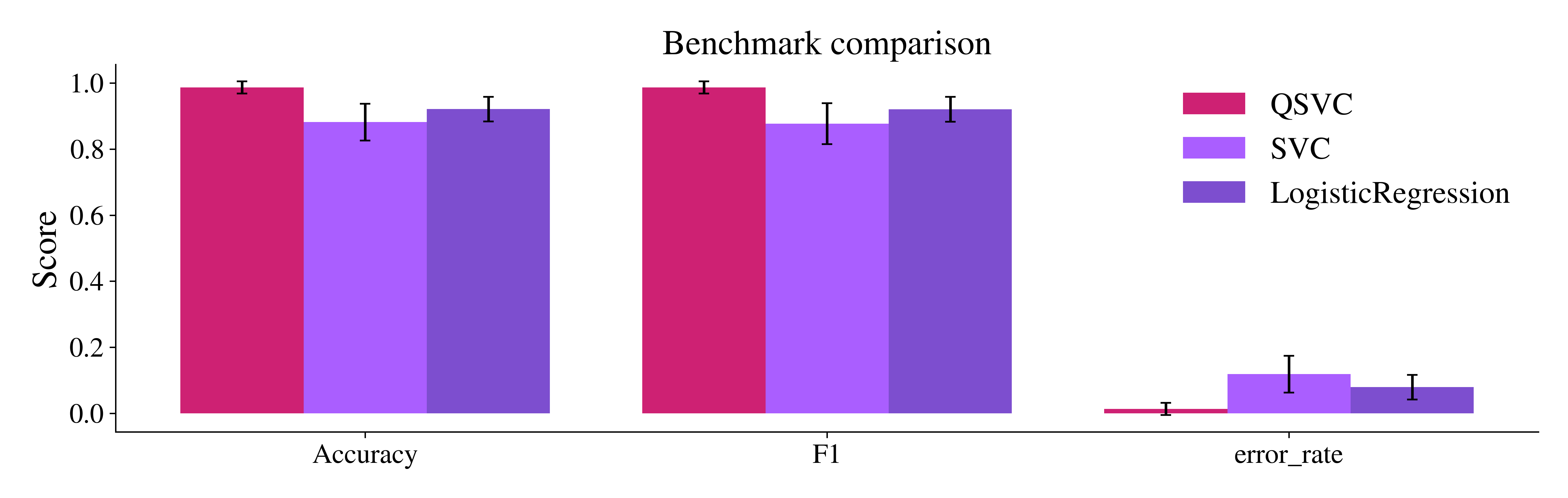
.plot() draws a grouped bar chart of the summary table. theme= chooses the
colours, and save_path= writes the figure to a file instead of showing it. One
loop therefore produces the two files that this page shows below. The site shows
the one that matches the reader's theme, and "dark" leaves the background
transparent:
for theme in ("light", "dark"):
    result.plot(save_path=f"{theme}_theme.png", theme=theme)

# Without `save_path` the same call shows the light figure inline.
result.plot()

Reuse the fitted result
best_model() returns the fitted estimator with the best mean score on the chosen metric. predict() is a shortcut that uses this selected model. Because the predictions were stored, the result can also build a confusion matrix without fitting again.
best = result.best_model(metric="accuracy")
preview_predictions = result.predict(X_preview, metric="accuracy")

print("Best model by accuracy:", type(best).__name__)
print("Predictions for five preview samples:", preview_predictions.tolist())
print("QSVC confusion matrix:")
print(result.confusion_matrix("QSVC"))
Best model by accuracy: QSVC
Predictions for five preview samples: [0, 1, 1, 1, 0]
QSVC confusion matrix:
[[12  0  0]
 [ 0 13  0]
 [ 0  1 12]]
Save numeric results
BenchmarkResult.save() writes the benchmark rows, the summary, the predictions, the paths of the saved models, the loss curves and the metric directions to a JSON file. It does not save the fitted estimators.